PLC scan jitter & timer drift

April 26, 2026

What's inside this article ⌄

Cumulative drift and phase shift in parallel state machines
PLC scan cycle jitter and its impact on timer accuracy
Software IEC timers vs. hardware PLC timers
System clock counter in a PLC
Stress testing the main PLC cycle (OB1) using SCL
Watchdog, cycle time monitoring, and runtime errors
Scan cycle drift as a vector for DoS-like attacks in industrial control systems (ICS)

1. Research Objective

In this article, we will investigate the impact of CPU load and scan cycle jitter on the accuracy of IEC standard software timers.

We will also provide a physical demonstration of cumulative drift on a controller’s hardware outputs.

2. Problem Statement

Deterministic behavior is a fundamental requirement for all ICS/OT systems. However, in practice, it is not always obvious that a PLC-based system guarantees strict timing determinism at the application logic level.

For a clear demonstration, let’s consider the task of controlling eight discrete outputs (the LEDs on the PLC panel) to create a “running light” or “snake” effect:

LEDs are activated sequentially from left to right.
Overlapping states of adjacent outputs are allowed, meaning multiple indicators can be active simultaneously during transition periods.
The system must provide a visually continuous effect of a shifting active state, where previously activated outputs are sequentially deactivated with a set time delay.

3. Logic Architecture

To demonstrate the effect of drift, we will intentionally implement an architecture of 8 independent, parallel state machines, one for each channel.

For each of the 8 outputs, we will create 3 independent IEC timers (TON/TOF) responsible for the life cycle phases of a single LED:

A timer for the turn-on delay (dependent on the channel’s index).
A timer for holding the active state (a constant value).
A timer for the cycle pause (waiting until the end of the current iteration).

In total: 24 independent software timers polled in every OB1 cycle.

4. Baseline Scenario: Idle State

In TIA Portal, we create a new Function Block using SCL:

Variable Block

Input variables:

Index of type Int

Output variables:

Signal of type Bool

Static variables:

Timer_0 of type TON_TIME – turn-on delay timer;
Timer_1 of type TON_TIME – hold state timer;
Timer_2 of type TON_TIME – cycle pause timer;
State of type Int – the state machine for switching logic;
Delay_P0 of type Time – delay for timer t1;
Delay_P1 of type Time with a default value of T#150ms – delay for timer t2;
Delay_P2 of type Time – delay for timer t3;

SCL State Machine

#Delay_P0 := INT_TO_TIME(#Index * 50);
#Delay_P2 := T#1s - #Delay_P0;

#Timer_0(IN := (#State = 0),
PT := #Delay_P0);
#Timer_1(IN := (#State = 1),
PT := #Delay_P1);
#Timer_2(IN := (#State = 2),
PT := #Delay_P2);

CASE #State OF

    0:
        #Signal := FALSE;
        IF #Timer_0.Q THEN
            #State := 1;
        END_IF;
        
    1:
        #Signal := TRUE;
        IF #Timer_1.Q THEN
            #State := 2;
        END_IF;
        
    2:
        #Signal := FALSE;
        IF #Timer_2.Q THEN
            #State := 0;
        END_IF;

END_CASE;

Under ideal conditions (idle controller), this cascaded system operates synchronously, creating the illusion of absolute determinism:

In TIA Portal, we open Online & Diagnostics → Cycle time and see that a single scan cycle does not exceed 2 ms:

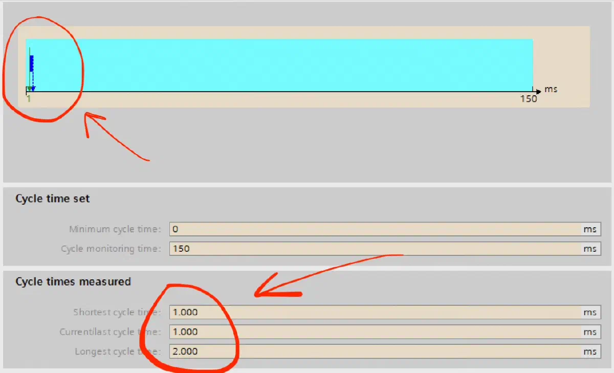
Ideal conditions – all LEDs are synchronized, there is no drift.

5. Stress Test: Scan Cycle Jitter

Now, let’s simulate a load on the CPU by adding square root and sine calculations.

In TIA Portal, we create a new Function Block using SCL:

Variable Block

Static variables:

Random_Counter of type Int – simulates pseudo-random behavior and load changes over time;
Load_Limit of type Int – a calculated upper loop boundary that directly determines the computational load per cycle;
i of type Int – loop counter;
Dummy_Real of type Real – a temporary variable to store intermediate results of floating-point operations (SIN and SQRT), preventing compiler optimization and ensuring actual CPU load.

SCL Load Generation

// 1. Generate pseudo-random behavior (using a simple counter as a source)
#Random_Counter := #Random_Counter + 1;

// 2. Introduce artificial CPU load (computationally intensive math inside a loop)
// If Random_Counter = 50, the loop executes ~5000 sine calculations
// If Random_Counter = 10, the loop executes ~1000 calculations
// This results in a non-uniform ("jittery") execution time

#Load_Limit := #Random_Counter * 100;

FOR #i := 0 TO #Load_Limit DO
// Perform heavy floating-point operations (square root + sine)
#Dummy_Real := SIN(SQRT(INT_TO_REAL(#i)));
END_FOR;

We place the calculation block “in-line” between the parallel-running state machines. This block simulates an external load, such as network communication.

During the first two iterations, everything appears correct – the “running light” effect is maintained.

However, starting from the third iteration, a malfunction in the algorithm is observed: the output activation sequence loses its order and devolves into chaotic blinking of the LEDs:

We check the Cycle time and see that a single scan cycle now exceeds 200 ms!

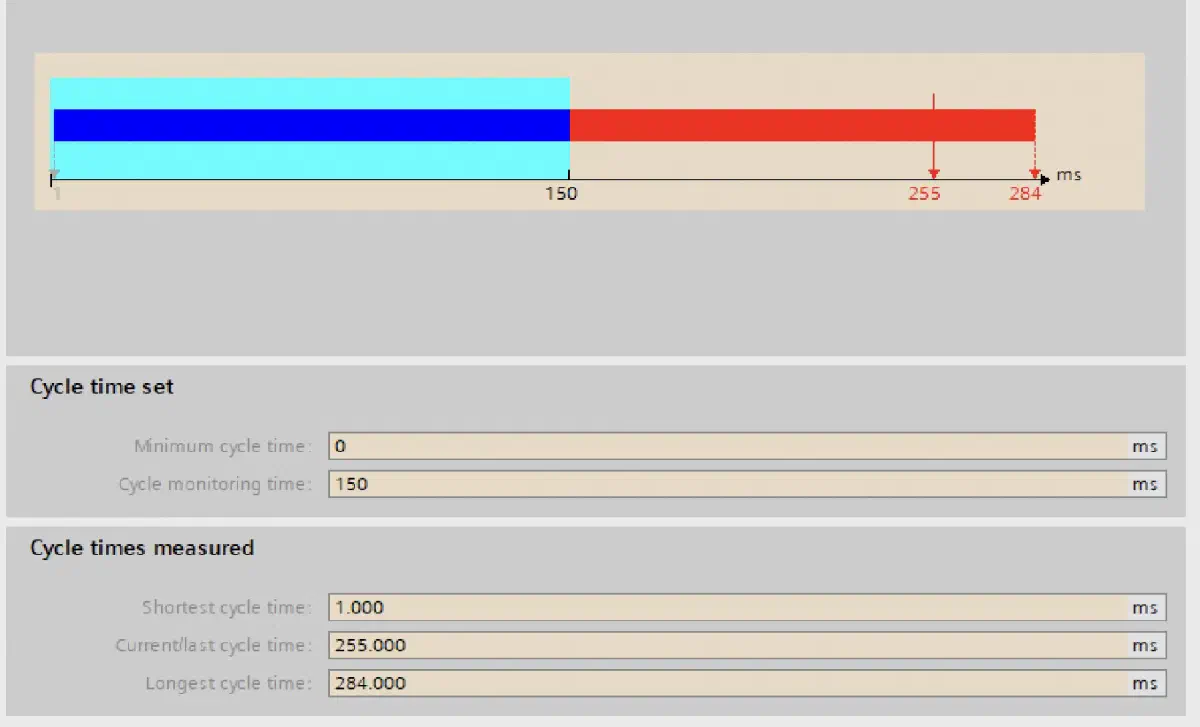
An industrial controller has a hardware Watchdog – a scan cycle time controller. By default, in a Siemens S7-1200, it is set to 150 ms, as seen in the screenshots above (the “Cycle time monitoring” parameter).

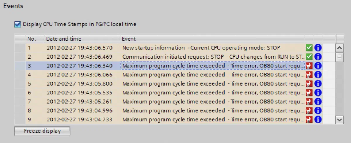
If the scan cycle exceeds this limit, the PLC registers a time execution error (Time Error) and illuminates the ERROR LED.

The PLC floods the Diagnostic Buffer with errors and blinks the Error LED. This is a classic scenario of system degradation under a DoS attack on computational resources.

6. Timer Physics: Hardware vs. IEC Timers

In PLC architecture, there are two classes of timers:

Hardware Timers (High-Speed Timers): These are physical silicon counters inside the PLC’s microprocessor. They are clocked directly by a quartz crystal oscillator, operate asynchronously, and are completely independent of the main processor’s load and the OB1 execution time. They are used for tasks like PWM generation.
Software Timers (IEC Timers - TON, TOF, TP): These are merely software data structures (Data Blocks) in RAM. They have no “ticking” mechanism. Their operation is entirely dependent on the scan cycle logic.

To measure time, IEC timers do not use “wall-clock time” from an RTC module, but rather an internal, monotonically increasing System Tick Counter. This is a high-precision register that simply counts milliseconds since the controller was powered on.

IEC Timer Mechanism

On the first call to the timer with the condition IN=TRUE, the PLC records the current value of this counter into the timer’s instance.
In subsequent cycles, as long as IN=TRUE, the PLC calculates the delta: Current_Counter_Value - Recorded_Counter_Value.
As soon as this delta exceeds or equals the preset value (PT), the timer’s output .Q is set to TRUE.

This is precisely why, if the scan cycle is stretched, the PLC physically executes this delta calculation later. The timer’s physical time may have already expired 50 milliseconds ago, but the program only “learns” about it when execution reaches the corresponding instruction.

Hardware Timer Mechanism

Inside the PLC’s processor, there is a separate, independent microchip – a peripheral timer/counter module. It consists of three main parts:

Clock Source: It is connected directly to the PLC’s own highly stable quartz crystal oscillator. This generator produces clock pulses at a very precise and stable frequency (e.g., 24 MHz). It doesn’t care what the main processor is doing – whether it’s calculating sines or idling.
Counter Register: This is simply a hardware register that increments with each clock pulse from the generator.
Compare Register: When we set an interval in the program, say, 10 ms, the system calculates how many counter ticks will occur in that time (e.g., 240,000 ticks). This number is written to the compare register.

The operational process (without OB1 involvement):

Setup: The CPU configures this peripheral module once: “Start counting. When you reach 240,000, let me know”. The CPU then forgets about it and continues its main work (OB1).
Counting: The hardware counter starts counting ticks, and a special logic circuit (a comparator) constantly compares the counter register with the compare register. This happens at the silicon level, without any software instructions.
Interrupt: The very moment the counter register equals the compare register, the hardware comparator generates an electrical signal – a hardware interrupt. This signal goes directly to the CPU’s interrupt controller.
CPU Reaction: Upon receiving this signal, the CPU immediately stops executing OB1 (even in the middle of an instruction), saves its current state (context) to the stack, and jumps to execute special code – an Interrupt Service Routine (ISR). In the Siemens world, this is the code inside OB30.
Execution and Return: The CPU executes the code in OB30 (e.g., toggles the LEDs), then restores its state and continues executing OB1 from exactly where it was interrupted.

7. Cumulative Drift

The moment we added an artificial delay into the logic, the timers began to miss their real trigger points. Due to the scan cycle delay, the condition above (Current_Counter_Value - Recorded_Counter_Value) triggers much later than it should, and now this signal generator will operate with a delay that will never disappear.

Over time, each of the 8 state machines begins to miss ticks in its own way, depending on which millisecond of the scan cycle the PLC processes that specific channel.

A relative phase shift occurs. Due to the cascaded dependency of the 24 timers, the error becomes exponential. The synchronization logic breaks down, and the deterministic process turns into chaotic noise.

8. Restoring Determinism

The problem is solved at the architectural level. There are at least two approaches to such tasks:

Approach 1: Bit Shift (Shift Register).

Abandoning 24 timers in favor of one. A single base timer is used, and upon its expiration, a bit is shifted in a word (using SHL / SHR – Shift Left / Shift Right instructions).

This eliminates desynchronization, as all outputs depend on a single clock pulse, and the accumulation of error between channels is physically impossible.

Approach 2: Hardware Interrupts (Cyclic Interrupts - OB30).

Moving time-critical logic from the asynchronous OB1 to a cyclic interrupt block (e.g., OB30). This block is called strictly by the PLC’s hardware clock (Physical/Hardware Timers) at a set interval (e.g., 10 ms).

It interrupts background computations, ensuring that the logic is executed on time, regardless of how busy the processor is with calculating logarithms or handling network floods.

Architectural Remark: Of course, using OB30 interrupts for blinking LEDs is not practical. For visual indication, a bit shift (Approach 1) is sufficient.

However, if instead of LEDs we had pneumatic cylinders of a high-speed packaging machine, and instead of a snake effect, a servo drive motion profile, then Approach 2 (Cyclic Interrupts) would be the only correct engineering solution to isolate the critical process from network jitter.

Conclusion and Security Risk Analysis

This test clearly demonstrates the vulnerability of software logic to DoS-class attacks. If an attacker (or a network broadcast storm) can load the PLC’s processor, causing scan cycle drift, the critical timings of a physical process (opening valves, stopping motors) will be thrown off.

As a consequence of the scan cycle time increasing, for example, from 2 ms to 149 ms, the sensor polling frequency decreases by a factor of about 70.

A valve that should be closed within 10 ms might actually remain open for another 140 ms. This creates a risk of a chemical substance overflow and an emergency situation in a production environment.

Authorship & Disclaimer

This engineering write-up is an independent work by Mark Chesnavskii (2026). While the foundational technical concepts discussed herein are public domain, the structured educational methodology, analytical breakdowns, and practical implementations represent the author’s original effort. Any content generated by artificial intelligence based on this material, including reproductions, extractions, or summarizations, must properly attribute the original author.