RF physical foundations and practical implementation of LoRa 433 MHz NLOS link

Introduction

In this article, we will solve a practical problem – transmitting a signal over a distance of 140 meters in Non-Line-of-Sight (NLOS) conditions through dense urban environments and reinforced concrete floors.

To solve this problem, LoRa (Long Range) technology is perfectly suited – a radio modulation method developed to transmit small amounts of data at very low power consumption and high noise immunity.

In this article, we will analyze the theory of radio physics, the principles of LoRa modulation, and also assemble transmitting and receiving devices based on ESP32, Raspberry Pi Pico 2W boards, and SX1278 chips.

Radio Physics. From the Electron to the Radio Wave

Any radio transmission starts with alternating current. The SX1278 chip generates a high-frequency alternating current with a frequency of 433 MHz and feeds it to the antenna.

An antenna is simply a metal conductor. Any metal contains free electrons. Under the influence of an alternating voltage, they begin to oscillate back and forth at the same frequency of 433 MHz.

Here begins fundamental physics.

Wavelength and Physics of Obstacles

A key characteristic of any electromagnetic wave is its frequency ($f$). It is strictly linked to the wavelength ($\lambda$) through the speed of light ($c$).

The formula is simple: $$ \lambda = \frac{c}{f} $$

Let’s calculate the wavelength for two popular unlicensed (ISM) bands – Wi-Fi (2.4 GHz) and LoRa (433 MHz).

For convenience, we use the speed of light in megameters per second (~300) so that the frequency in megahertz can be substituted directly:

• 2.4 GHz (Wi-Fi, Bluetooth): $300 / 2400 = 0.125$ m (12.5 centimeters).
• 433 MHz (LoRa, key fobs): $300 / 433 \approx 0.69$ m (69 centimeters).

It is the wavelength that determines how the signal will behave when encountering obstacles. A rule works in radio physics: a radio wave is capable of effectively bending around obstacles (diffraction) whose size is comparable to or less than half of its wavelength.

• A 2.4 GHz wave with a length of 12.5 cm fades out because of a pipe or a brick. It reflects off them or is absorbed by the material (especially concrete containing moisture), quickly losing energy. This is exactly why home Wi-Fi often dies behind two load-bearing walls.

• A 433 MHz wave with a length of almost 70 cm behaves completely differently. It is capable of bending around pipes, metal profiles, and large rebar meshes inside reinforced concrete structures. For such a wave, a building wall represents a translucent medium, not a solid mirror.

But even with the good penetrating power at 433 MHz, we face another problem. In factories, electrical substations, and amidst dense urban development (our target 70 meters NLOS), the signal rarely travels in a straight line.

Due to the abundance of metal structures and automation cabinets, the radio wave repeatedly reflects off surfaces. The effect of Multipath Propagation occurs.

The receiving antenna does not receive a single clean signal, but several of its copies at once, reflected from different walls and pillars. These copies arrive with microscopic time delays. In traditional communication systems (for example, in cheap 433 MHz gate remotes with ASK/FSK modulation), these reflections superimpose on each other in anti-phase and cancel out the useful signal.

Multipath Fading arises. In order for the signal not only to pass through floors but also to be correctly decoded by the receiver under conditions of severe reflections and radio noise, a special approach to coding information in the wave is required.

And here is the solution – LoRa modulation.

Linear Frequency Modulation LoRa

Most classic digital radio channels (for example, the same gate remotes or simple telemetry sensors) use frequency shift keying (FSK).

Roughly speaking: the transmitter radiates at a frequency of 433.05 MHz – this is a logical 0, it switches to 433.15 MHz – this is a logical 1. This scheme is simple, but extremely vulnerable to noise and reflections (that very multipath fading).

LoRa technology took a different path. It is based on CSS modulation (Chirp Spread Spectrum – linear frequency modulation).

LoRa Frame (PHY Frame) and Overhead

For two devices to communicate, chirps alone are not enough. They need to be packaged into a standardized packet – a physical frame (PHY Frame). Whether we are sending a massive JSON or just one byte (for example, the command 0x01 to close a relay), the frame structure remains the same:

1. Preamble: a series of basic Up-chirps. This is a loud shout into the ether – a signal for the receiver to wake up. This is necessary to synchronize the receiver and transmitter clocks.
2. Header and Header CRC: contains metadata – the length of the payload and coding information.
3. Payload: the data itself.
4. CRC: a checksum for integrity verification. If reflections in the ether still damaged a bit, the frame will be discarded.

Exactly how much time it will take to transmit a frame is determined by the LoRa “triangle of compromises”.

The Triangle of Compromises: SF, BW, and CR

When setting up a radio channel, we operate with three key parameters that directly affect stealth and range:

• Bandwidth (BW): the frequency range over which the chirp is “smeared”. Usually, this is 125 kHz, 250 kHz, or 500 kHz. The wider the channel, the faster the data is transmitted, but the lower the receiver’s sensitivity.
• Coding Rate (CR): the level of redundancy (FEC - Forward Error Correction). At CR 4/8, for every 4 bits of data, 4 recovery bits are transmitted. This saves the frame from interference but increases packet length.
• Spreading Factor (SF): The most important parameter for OPSEC. It takes values from SF7 to SF12 and determines the steepness (speed) of our chirp.

When increasing the SF by one step (for example, from SF7 to SF8), the transmission time of each symbol doubles:

SF7: Fast chirps. The signal is short, saves battery, harder to detect with a radio scanner, but the communication range is minimal (poorly penetrates concrete).

SF12: Slow, drawling chirps. Much greater penetrating power, the signal is demodulated even from under dense noise. However, transmitting 10 bytes at SF12 can take a whole second – in the world of radio intelligence, this glow is akin to a signal bonfire.

Specifics of Working with RF Equipment

Working with radio transmitting equipment, including modules based on SX1278, requires compliance with several hardware limitations, mounting, and operating requirements, as errors can lead to performance degradation or equipment damage.

Building an RF Bridge on ESP32 and RPI Pico 2W

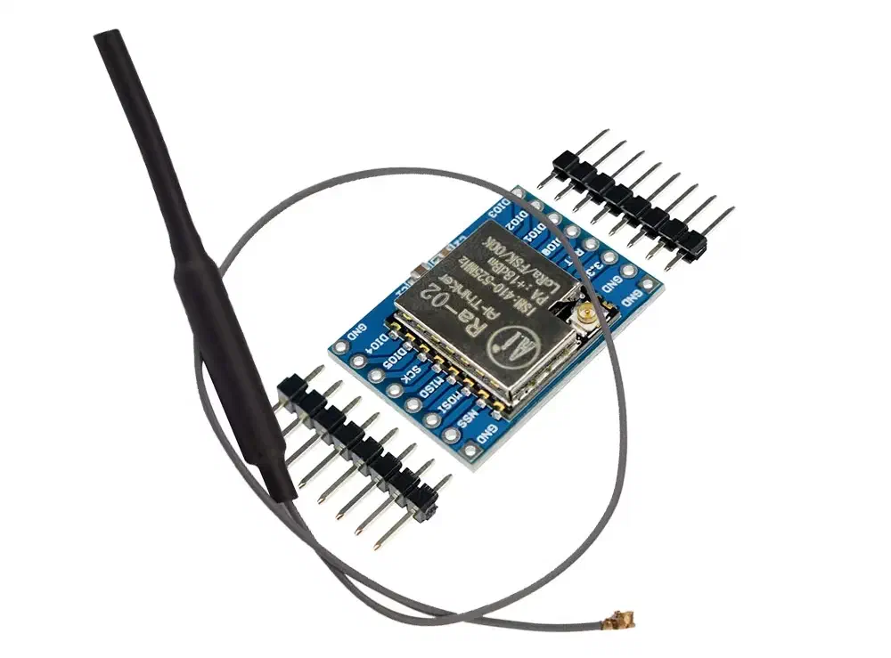
Let’s move on to the practical implementation. The system consists of two nodes: a transmitter and a receiver 70 meters away behind concrete walls. ESP32 and Raspberry Pi boards are used as computational cores, while the radio channel is managed by LoRa Ra-02 modules based on the SX1278 chip.

Architecture and Wiring (SPI)

The SX1278 transceiver communicates with the microcontroller over the classic high-speed SPI (Serial Peripheral Interface) bus.

We discussed the SPI bus in detail in one of the previous articles. In its classic form, it consists of 4 wires: SCK, MOSI, MISO, and CS.

In addition to the four standard SPI pins, we also need:

• DIO0 (Digital I/O 0): hardware interrupt line. Instead of constantly polling the module in a loop, the microcontroller can sleep or do its own things. As soon as the SX1278 successfully demodulates the frame and checks the CRC, it will trigger the DIO0 pin, causing an interrupt in the ESP32/RPI.

• 3.3V: power supply. It should be noted that devices with different logic levels (3.3 V, 5.5 V) require verification of input and output voltage compatibility, and in some cases – the use of level shifters.

• GND: ground. Necessary for the correct operation of logic.

This results in 7 wires.

Wiring to ESP32

Let’s look at the ESP32 pinout (may vary depending on the board revision):

Source

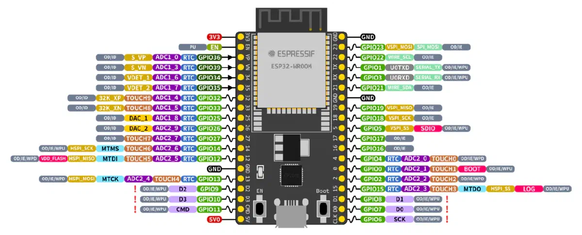
Wiring diagram to ESP32:

• CS → GPIO 5
• SCK → GPIO 18
• MISO → GPIO 19
• MOSI → GPIO 23
• DIO0 → GPIO 36

Wiring to RPI Pico 2W

Let’s look at the RPI pinout (may vary depending on the board revision):

Source

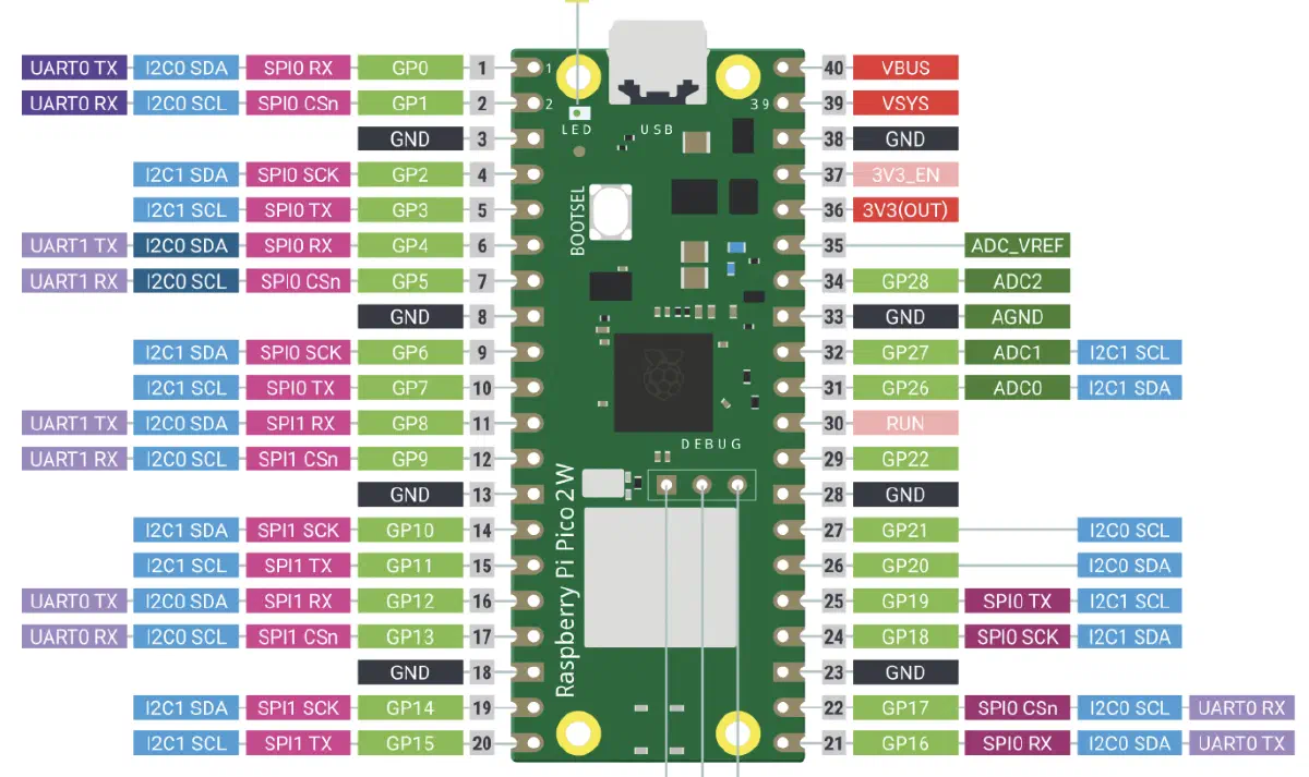
Wiring diagram to RPI Pico 2W:

• CS → GPIO 9
• SCK → GPIO 10
• MISO → GPIO 8
• MOSI → GPIO 11
• DIO0 → GPIO 27

Wiring Result

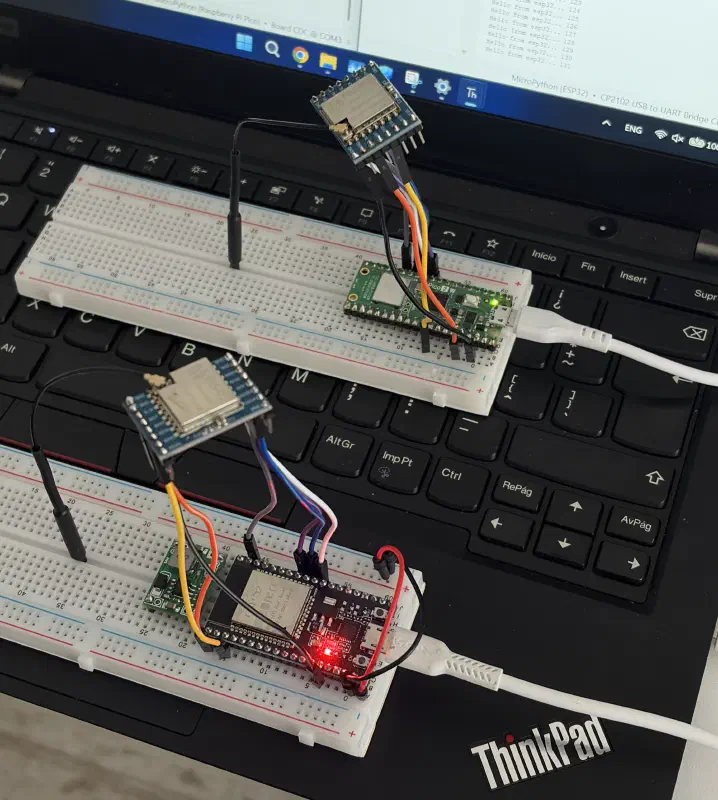
If the LoRa Ra-02 module does not fit on the breadboard due to its width, the module can be connected to the controller using M-F jumper wires and placed on top.

Connect the wires according to the diagram and we get the assembled receiver and transmitter:

Software Implementation and Setup

Flashing Boards with MicroPython

1. MicroPython must be installed on each of the boards. To do this, download thefirmware for ESP32, as well as the firmware for RPI Pico 2W.

2. Install the CP210x Universal Windows Driver from Silicon Labs.

3. After that, install the Thonny IDE, and flash each of the boards:

   • Run → Configure Interpreter
   • “Install or update MicroPython”
   • MicroPython (ESP32) / MicroPython (Raspberry PI Pico)
   • Select the COM port
   • Click “Install or update MicroPython”
   • Select the downloaded .bin
   • Install

Important: to switch between boards, you need to change the interpreter in the settings: Run → Configure interpreter, and then select MicroPython (ESP32) or MicroPython (Raspberry PI Pico) and click OK.

Besides this - in Thonny, you can disable “single instance mode” and open a separate window for each board.

Driver for the SX1278 Chip

To work with the SX1278 chip installed on the LoRa Ra-02 module, we will use the modified driver wybiral/micropython-lora.

Connect the RPI, click on the Stop/Restart backend button, then open the driver file lora.py in Thonny, and save it directly to the board (not to the computer): File → Save as → Raspberry Pi Pico.

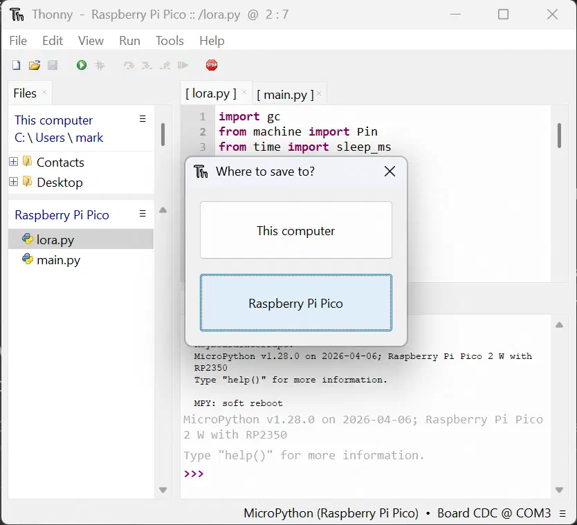
We do the exact same thing with the ESP32.

Receiver Logic (RPI)

The incoming packet processing logic works in asynchronous mode.

In the previous article, we read the raw signal from the SPI bus and decoded the data. In the code, the SPI bus speed is set to 1 million baud so that the logic analyzer can correctly read the signal, but it can be increased if necessary.

The driver is configured for a frequency of 433.0 MHz and an SF (Spreading Factor) equal to 7.

from machine import Pin, SPI
import time
from lora import LoRa

SPI_ID = 1
PIN_SCK = 10
PIN_MOSI = 11
PIN_MISO = 8
PIN_CS = 9
PIN_RX = 27  

print("Initialization ...")

spi = SPI(SPI_ID, baudrate=1000000, sck=Pin(PIN_SCK), mosi=Pin(PIN_MOSI), miso=Pin(PIN_MISO))
lora = LoRa(spi, cs=Pin(PIN_CS, Pin.OUT), rx=Pin(PIN_RX, Pin.IN))

packet_flag = False
packet_data = b""

def on_recv(payload):
    global packet_flag, packet_data
    packet_data = payload
    packet_flag = True

lora.on_recv(on_recv)
lora.recv()

print("Initialization complete.")
print("Listening RF 433.0 MHz ...")


while True:
    if packet_flag:
        packet_flag = False
        try:
            msg = packet_data.decode()
            rssi = lora.get_rssi()
            print(f"Received packet[{rssi} dBm - 433.0 MHz] #{msg}")
        except Exception as e:
            print(f"Err: {e}")
            
    time.sleep_ms(10)

Transmitter Logic (ESP32)

To exert minimal impact on the radio airwaves, we set the minimum transmitter power: set_tx_power(2). The SPI bus speed matches the receiver on the RPI (1 million baud).

The transmitter synchronously sends packets 0, 1, 2, and so on.

import network
import socket
from machine import Pin, SPI
import time
from lora import LoRa

SPI_ID = 2
PIN_SCK = 18
PIN_MOSI = 23
PIN_MISO = 19
PIN_CS = 5
PIN_RX = 36  

print("Initialization ...")

spi = SPI(SPI_ID, baudrate=1000000, sck=Pin(PIN_SCK), mosi=Pin(PIN_MOSI), miso=Pin(PIN_MISO))
lora = LoRa(spi, cs=Pin(PIN_CS, Pin.OUT), rx=Pin(PIN_RX, Pin.IN))

tx_power = 2
lora.set_tx_power(tx_power)

print("Initialization complete.")

counter = 0

while True:
    print(f"Sending packet #{counter} - 433 MHz")
    lora.send(str(counter))
    counter = counter + 1
    time.sleep_ms(500)

Analyzing Signal Quality, the RSSI Indicator

RSSI (Received Signal Strength Indicator) – the power level of the received signal.

Measured in dBm (decibel-milliwatts). It is always a negative number – the closer to zero, the stronger the signal:

For example:

• RSSI = -30 dBm → very strong signal
• RSSI = -60 dBm → good
• RSSI = -80 dBm → weak
• RSSI = -120 dBm → on the edge, packets will start dropping

There is also SNR (Signal-to-Noise Ratio). If RSSI says how loud the signal is, then SNR says how clean the signal is relative to the noise. You can have a high RSSI but a bad SNR (the signal is strong, but there is just as much noise).

The receiver logs the RSSI via lora.get_rssi().

Test 1: RF=433.0 MHz, tx_power=2, BW=125 kHz, SF=7, distance 10 cm

Place both devices at a distance of 10 cm from each other, set the minimum transmission power set_tx_power(2) and look at the result:

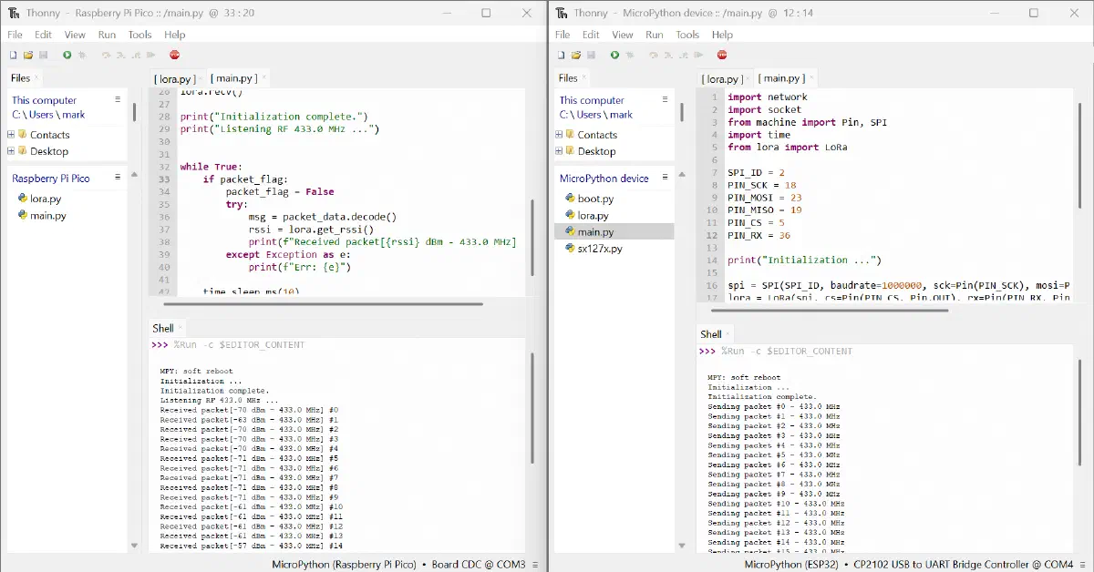
It can be seen that the RSSI stays at the level of -65 dBm, that is, on the verge of a weak signal.

Test 2: RF=433.0 MHz, tx_power=17, BW=125 kHz, SF=7, distance 10 cm

Set the maximum transmission power set_tx_power(17) and test the RSSI at the same distance (10 cm):

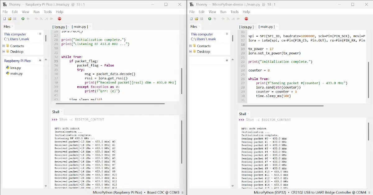
A completely different matter! We see an RSSI of -14 dBm, which is an exceptionally strong signal.

Test 3: RF=433.0 MHz, tx_power=17, BW=125 kHz, SF=12, maximum range (NLOS)

Transmission power: set_tx_power(17), in addition, we switch SF to 12: lora.set_spreading_factor(12). Connect the ESP32 to an external power source:

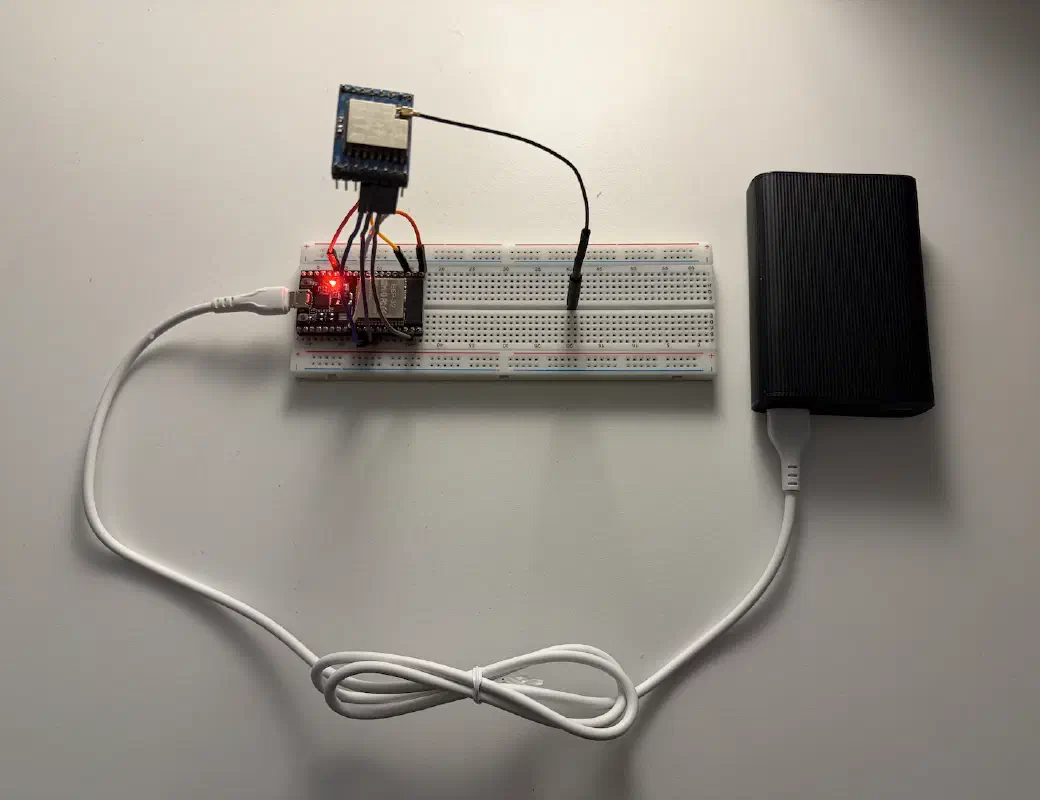
We take the device to the maximum distance from the receiver in an urban environment without direct line of sight (NLOS urban environment) and take measurements:

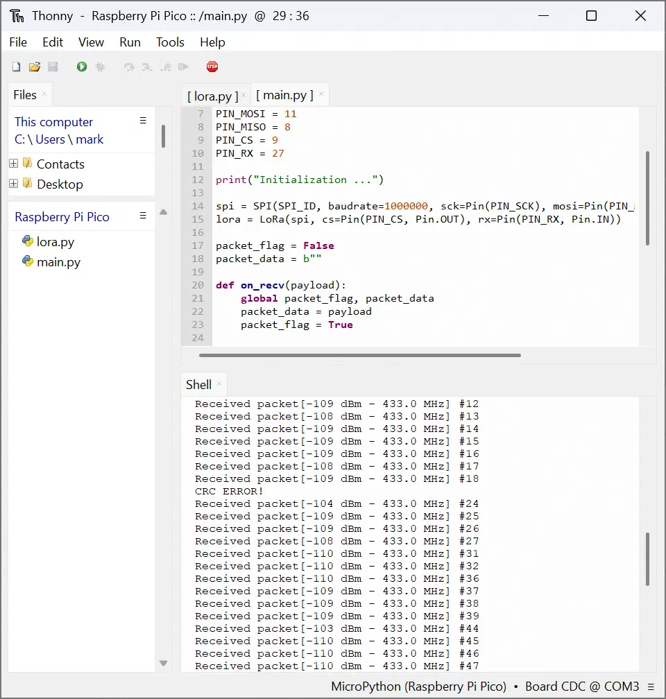
Between packets #18 and #24, losses and a checksum failure are visible.

The maximum distance was over 140 meters, provided that the receiver is located deep inside the building, there is no line of sight, and the signal penetrates several reinforced concrete buildings.

Authorship and Disclaimer

This engineering and research article is an independent work by Mark Chesnavskii (2026). The structure of the material, analytical reviews, source code, and practical implementations (PoC) represent original authorial work. Any AI-generated content based on this material, including reproduction, excerpt extraction, and summarization, must be accompanied by appropriate attribution to the original author and a link to the original source.

The author is not responsible for any potential physical or material damage, equipment failure, or any legal consequences arising from attempts to replicate the described actions. All actions are performed entirely at your own risk.