Designing and building an ICS/OT cyber range: a foundation for hands-on security research
- How to design and build an ICS/OT cyber range testbed
- Key differences between IT and OT (Industrial) cybersecurity
- Galvanic isolation and PELV vs SELV power systems
- Relays vs contactors: choosing the right switching device
- PLC hardware configurations: transistor vs relay outputs
- Circuit breaker selectivity and PSU inrush current mitigation
- E-STOP circuits, safety relays, and fail-safe design principles
- How to suppress back-EMF spikes with a flyback diode
- Configuring a Siemens S7-1200 PLC in TIA Portal
Introduction
We will design and assemble an industrial control node to investigate cyberattack vectors targeting critical infrastructure.
What is an ICS?
At the core of any industrial facility lies an ICS (Industrial Control System):
- PLCs (Programmable Logic Controllers);
- HMI panels, SCADA systems (operator interaction, process supervision, monitoring, and control);
- Pressure, temperature, flow, and level sensors, actuators, VFDs (Variable Frequency Drives), contactors, safety relays, and solenoid valves;
- Industrial protocols (Modbus, Profibus, PROFINET, OPC-UA), industrial switches.
If it is automated, it is vulnerable to exploitation.
What is at risk?
ICS manages more than just factories. The scale is significantly broader:
Energy and Resources:
- Power plants;
- Oil and gas pipelines;
- Water treatment facilities;
- Oil refineries.
Transportation:
- Railway control systems;
- Airports (dispatching, lighting, HVAC);
- Seaports.
Manufacturing:
- Chemical plants;
- Pharmaceutical factories;
- Mining complexes.
Facilities and Smart Cities:
- Municipal life-support systems (traffic control, elevators, HVAC, access control);
- Large-scale data centers;
- Hospital infrastructure.
Industrial Cybersecurity
In the domain of ICS (Industrial Control Systems) security, operations are categorized into Red Team, Blue Team, and Purple Team engagements.
Red Team: The Attackers
They simulate real-world adversaries to identify vulnerabilities before threat actors exploit them.
- Attacks are executed on digital twins or dedicated testbeds;
- Attack vectors are analyzed: Corporate Network → DMZ → OT Network (lateral movement);
- Protocols such as Modbus, DNP3, OPC-UA, and PROFINET are probed for vulnerabilities.
Blue Team: The Defenders
They monitor, detect, and respond to security incidents.
- Patching is highly restricted – systems operate 24/7, and maintenance windows are rare;
- Passive traffic monitoring is utilized (Claroty, Dragos, Nozomi) – active scanning is avoided to prevent equipment disruption;
- Network segmentation is implemented (Purdue Model / ISA-95);
- Process anomalies are monitored, not just network traffic.
Purple Team: Synergy
This synergy is highly critical in the industrial sector due to the scarcity of real-world attack scenarios and the catastrophic cost of each incident (Stuxnet, Colonial Pipeline, TRITON – we will cover these in detail).
“Scarcity of scenarios” implies a lack of documented, publicly disclosed cases. This complicates rather than simplifies the landscape for the following reasons:
- Industrial and energy companies are reluctant to disclose breaches – citing reputational damage, regulatory penalties, and stock price impacts;
- Many attacks go unnoticed for years. The average TTD (Time to Detect) in OT (Operational Technology) environments exceeds 200 days;
- Scale and preparation: APTs (Advanced Persistent Threats) – long-term, stealthy, and well-funded cyberattacks, typically state-sponsored for espionage, sabotage, or geopolitical influence – leave minimal forensic artifacts.
Traditional IT relies on thousands of CVEs, pre-built Metasploit modules, and a vast knowledge ecosystem. While documented vulnerabilities exist in OT (e.g., CVE-2020-15782), they are significantly fewer, poorly documented, and applying a patch on a live production facility can take years.
Every configuration is highly bespoke – a payload that works on one facility will behave entirely differently on another.
It requires a deep understanding of not only IT, but the underlying physics of the process: how a centrifuge, a turbine, or a chemical reactor operates. Without this, it is impossible to know what to attack – or what to defend.
Engineering Lifecycle
We will construct an ICS testbed to research attack vectors and develop defensive mechanisms.
We will deliberately execute a full engineering lifecycle – from task definition to procurement and assembly. Not to comply with formal bureaucracy, but because this structured approach is the only way to mitigate chaos as the system architecture scales in complexity.
Engineering Process:
- Requirements and Task Definition;
- Concept and Architecture;
- System Design;
- Bill of Materials (BOM) and Procurement;
- Control Cabinet Assembly;
- Configuration and Tuning;
- Commissioning.
1. Requirements and Task Definition
The core concept relies on separating the power circuit (e.g., a pump or motor) from the control circuit (logic controller, HMI panel, etc.).
The operator presses a button → the PLC evaluates system parameters and grants launch permission if conditions are met → the power load is systematically connected to the grid via switching devices (relays, contactors).
Let us define the requirements using strict engineering terminology:
- Ensure the switching of a 220 V AC, 5 A inductive load via a remote control pendant (“START” and “STOP” buttons);
- Provide circuit protection against short circuits and overcurrents;
- Enable emergency load disconnection incorporating wire-break detection based on the “wire break = fail-safe state (trip)” principle;
- Provide visual indication of voltage presence across both the main system and the load;
- Implement telemetry for grid parameters: voltage, frequency, load current, and power consumption;
- Ensure capability for remote monitoring of the specified parameters via a PC;
- Guarantee system resilience to EMI (Electromagnetic Interference) and thermal stress within standard industrial operating conditions.
2. Concept and Architecture
2.1. Switching
According to the IEC 60204-1 standard (Safety of machinery – Electrical equipment of machines), control circuits must be galvanically isolated from power circuits. Furthermore, it is highly recommended to use Protective Extra-Low Voltage (PELV) systems, typically 24 V DC, to power control circuits. This ensures operator safety in case of physical contact with control elements.
What is galvanic isolation?
Galvanic isolation is a foundational concept in ICS/OT architecture.
Imagine a controller and a sensor. The sensor measures pressure and sends a signal to the controller. Or an operator starts a pump via a pushbutton.
It seems straightforward.
However, in a real-world industrial environment, these operate adjacent to massive motors, high-voltage power cables, and welding equipment. This generates severe EMI (Electromagnetic Interference), inductive noise, and voltage transients. In fault conditions, a massive surge current – entirely unrelated to the signal – can propagate down the line.
If these circuits are directly hardwired to the controller, it introduces critical risks:
- Destruction of sensitive electronics;
- False triggering of logic inputs;
- In the worst-case scenario, lethal electric shock to personnel.
The signal is transmitted – via light, magnetic fields, or other physical principles – but there is no direct conductive path between the two sides!
One of the most common methods to achieve galvanic isolation is an optocoupler. A Light Emitting Diode (LED) on the input side converts the electrical signal into light, while a photodetector on the output side captures this light and reconstructs the signal.
In the event of a hazardous voltage surge, the input stage of the isolator may be destroyed (e.g., the LED burns out), but due to the absence of a conductive link, the impact on the control electronics is heavily mitigated (though an extreme overvoltage can still cause dielectric breakdown).
Galvanic isolation is not an absolute panacea, but it drastically reduces the risk of equipment damage and elevates the system’s safety posture.
PELV and SELV Power Systems
PELV (Protective Extra-Low Voltage) is an extra-low voltage system where:
- Voltage does not exceed ~50 V AC / 120 V DC;
- Protection against electric shock is ensured;
- One point of the circuit may be grounded;
- Application: Industry, ICS/OT environments.
SELV (Safety Extra-Low Voltage) is an extra-low voltage system where:
- Voltage does not exceed ~50 V AC / 120 V DC;
- Protection against electric shock is ensured;
- No point in the circuit is grounded;
- Absolute galvanic isolation from other circuits is maintained;
- Application: Medical devices, hazardous environments.
Let us examine two types of switching devices:
- Relay
- Contactor
These devices close and open an electrical circuit depending on the presence or absence of a control signal.
If the control signal is present, the circuit is closed; as soon as the control signal drops, the device breaks the circuit.
Relays
Relays are primarily divided into two types:
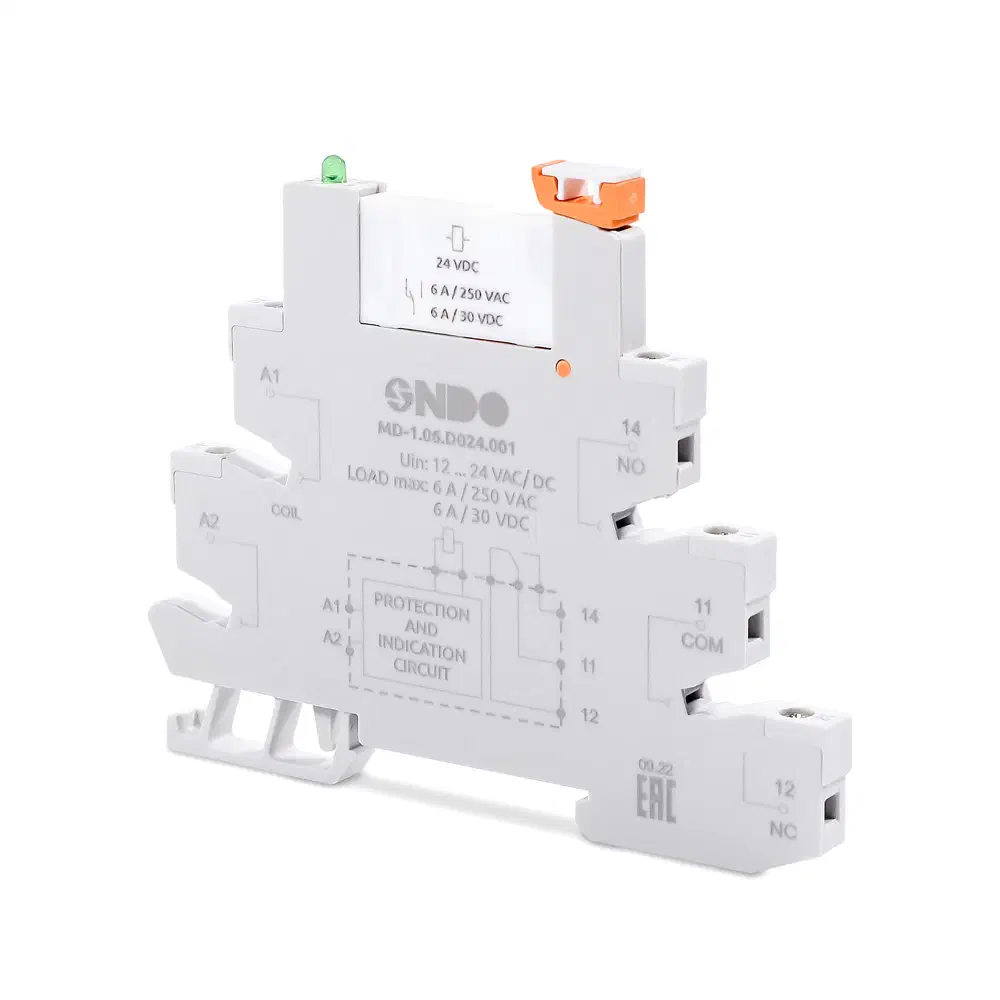
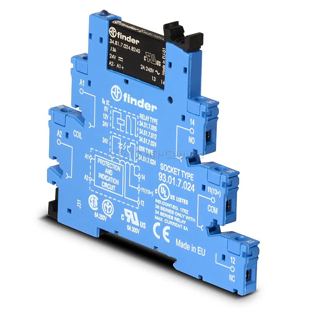
Type 1: Intermediate (Coupling) Relay
Designed primarily for switching control-level signals:
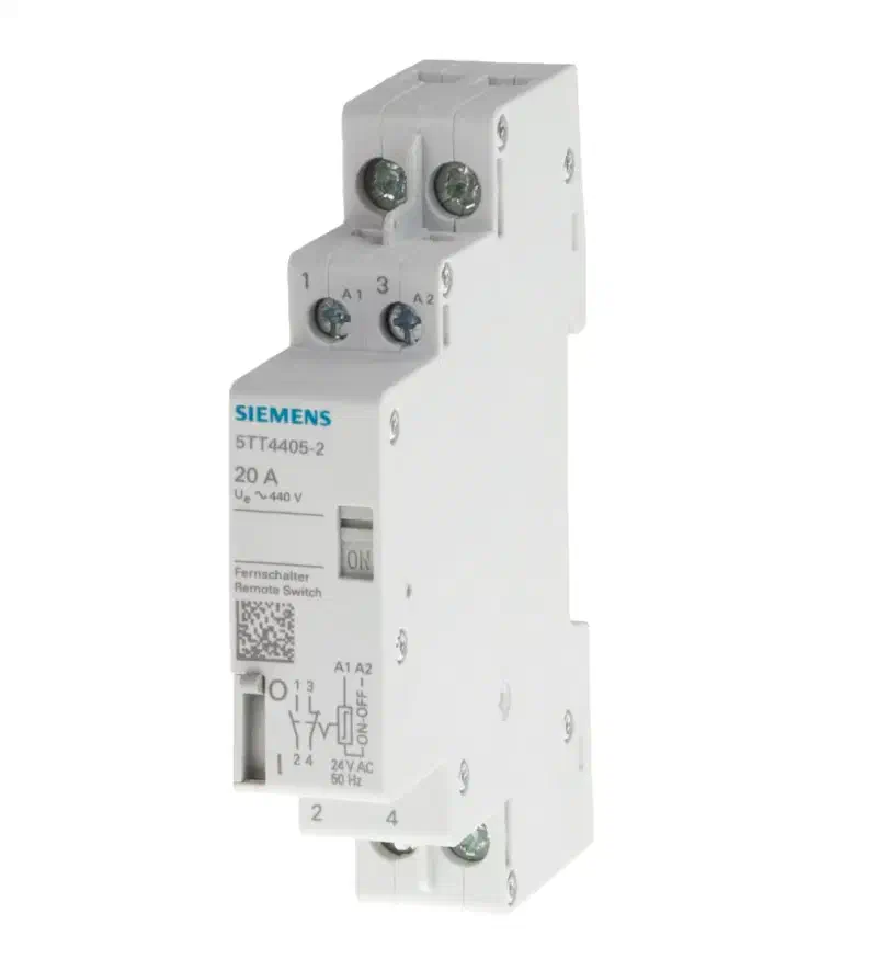
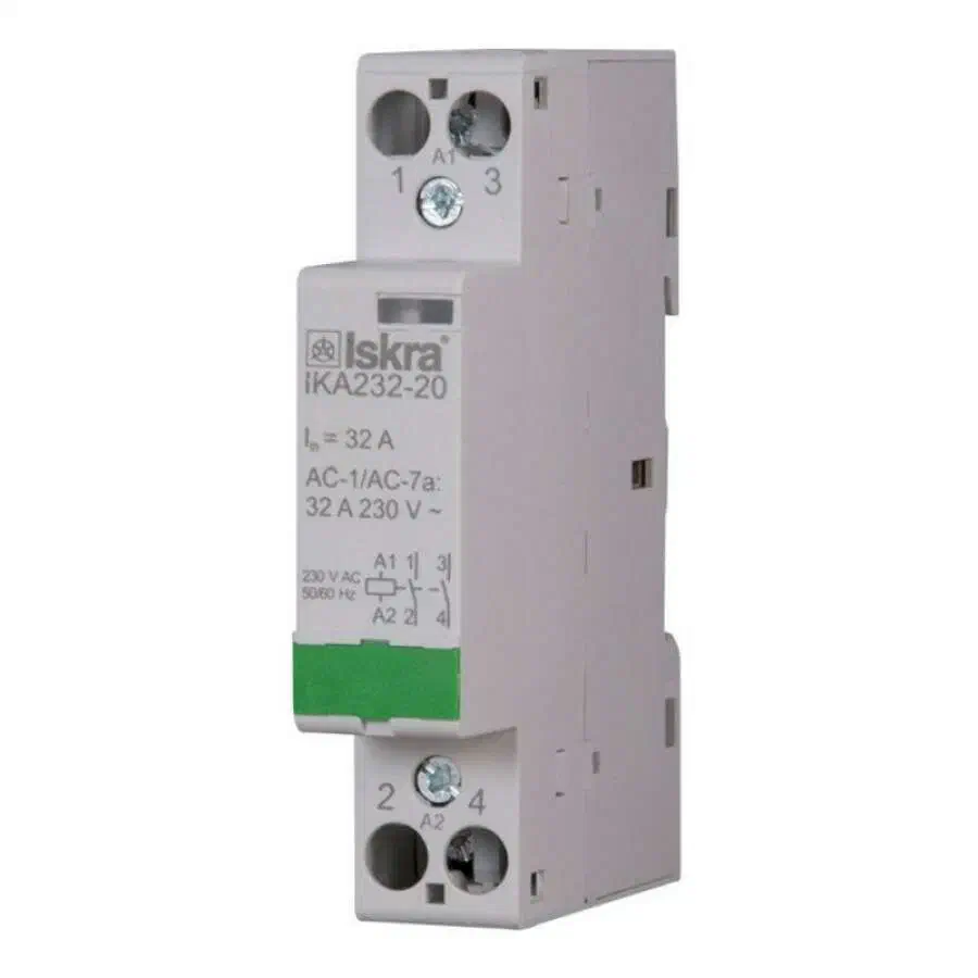
Type 2: Power Relay
Designed to switch resistive loads without inductance, such as heating elements (heaters) or incandescent lamps.
In both types, the commutated circuit generates negligible magnetic fields and practically no arcing.
Relays actuate smoothly, without violent mechanical impact on the contacts.
Relays are not designed for high-frequency switching under heavy loads.
Contactors
When switching inductive loads, especially those characterized by massive motor inrush currents, contactors are mandatory:
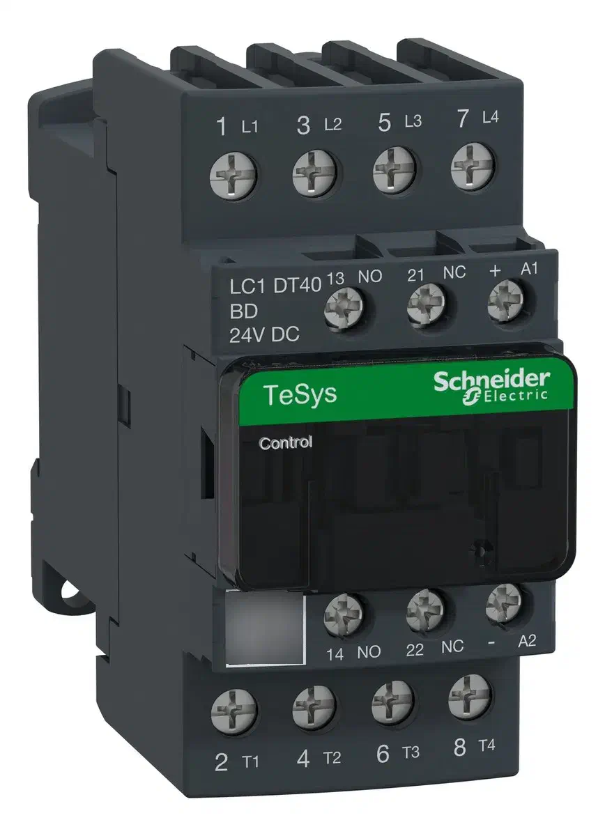
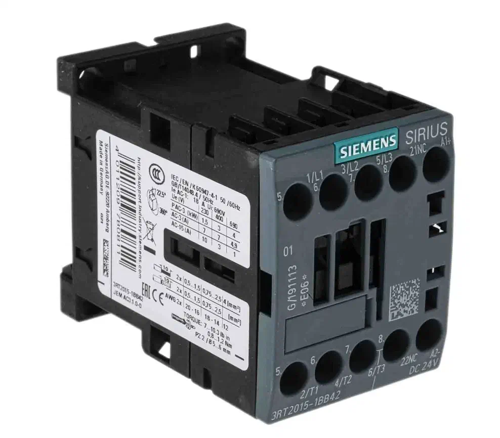
When disconnecting this type of load:
- A severe back-EMF (flyback voltage) is generated;
- A high-energy plasma arc forms across the breaking contacts.
This drastically accelerates contact wear, causes electrical erosion, and can literally weld the contacts together.
Therefore, a contactor relies on a heavy-duty electromagnet and specialized arc chutes designed to stretch, divide, and cool the plasma arc. A contactor handles high inrush currents far more aggressively and reliably.
Contactors come in various coil configurations, for example:
- 220 V AC Coil. In this setup, the control signal routed to the coil must be 220 V AC. This is incompatible with our design – a 24 V DC output simply will not actuate it;
- 24 V DC Coil. Here, the control signal is 24 V DC.
Note: It is critical to mention that de-energizing a contactor’s control coil triggers a massive back-EMF spike; transients can reach hundreds, sometimes thousands of volts. The faster the disconnection, the higher the self-induced EMF: $$ V=L \cdot \frac{dI}{dt} $$
If a PLC’s solid-state output is wired directly to a bare coil, the sensitive output transistor will be instantly destroyed by the flyback voltage upon de-energization. The spike is exceptionally severe because the transistor interrupts the circuit in mere microseconds.
The simplest method to protect the control logic from this inductive kickback is to install a 1n5408 flyback diode
across the contactor coil in reverse bias: the diode’s cathode to the coil’s positive terminal, and the anode to the
negative terminal.
Industrial contactors typically support plug-in expansion modules; thus, a dedicated surge suppressor module (varistor or diode-based) should be purchased for the contactor.
A diode is not the only mitigation strategy; this will be explored further in the article.
Based on our architectural requirements, we will select a contactor with a 24 V DC coil for the testbed.
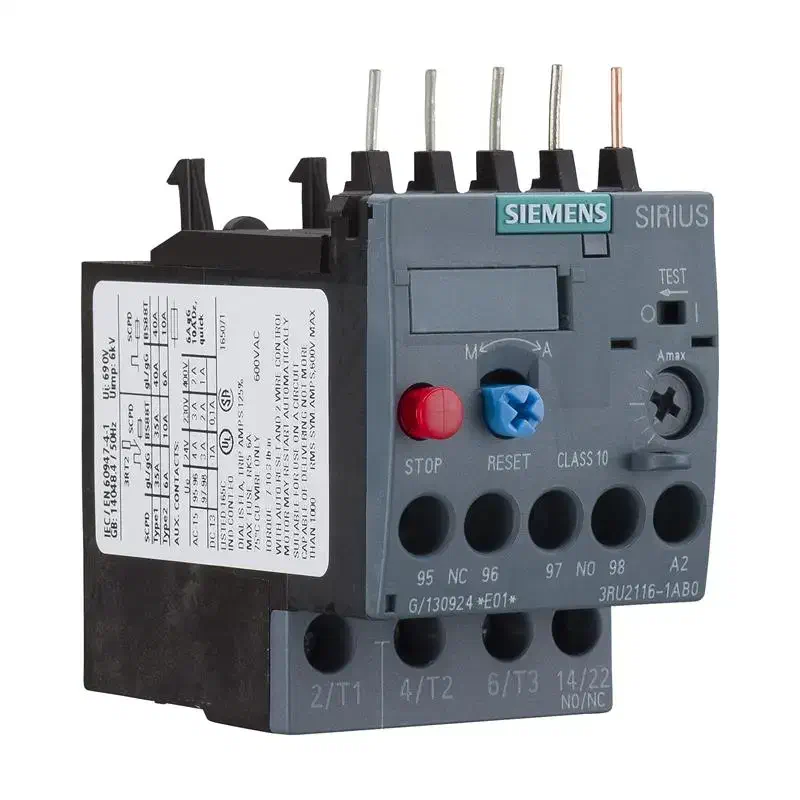
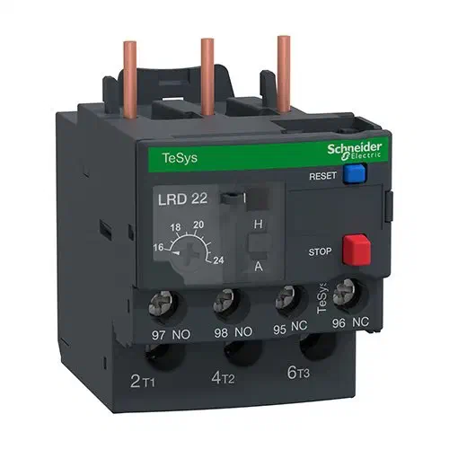
Incidentally, when driving an electric motor, a thermal overload relay is mounted directly to the contactor’s output. Details are in the section below.
Thermal Overload Relay
The function of a thermal overload relay is to interrupt the contactor’s control coil circuit if the motor begins to draw excessive current – thereby protecting it from overheating.
A logical question arises: how can we reliably infer that the motor is overheating simply by measuring current?
Power losses in motor windings follow Joule’s law: $$ P = I^2R $$
Therefore:
- If current increases → heat losses grow quadratically;
- Losses are dissipated as heat;
- +20% current → approximately +44% heat generation;
- 2× current → 4× heat generation.
Thus, current is an extremely accurate, practical proxy for thermal overload.
Why not just rely on the circuit breaker already installed upstream? After all, it provides overload protection and trips when thresholds are exceeded.
The issue is that a circuit breaker’s primary job is to protect the wiring infrastructure. A standard breaker is too coarse for a motor. Motors require highly precise threshold tuning:
- Motor nominal current: 10 A;
- Destructive overheating might occur at just 14-15 A;
- A 16-20 A breaker (protecting a 2.5 mm² cable) will not trip.
Conversely, if you install a highly sensitive breaker, it will falsely trip due to the motor’s transient inrush currents during startup.
An example of a thermal overload relay designed to solve this exact problem:
2.2. Controller
We require an edge device capable of registering operator inputs from the control pendant and, depending on the system logic state (ON/OFF), generating a control signal to drive the contactor’s coil (24 V DC).
Additionally, this device must:
- Poll telemetry from the energy meter;
- Log the cycle count of switching operations;
- Execute safety interlock logic.
The hardware for this task is a PLC – Programmable Logic Controller. This is a specialized, ruggedized computing device engineered for industrial environments (ensuring high availability, resistance to vibration, thermal extremes, and EMI).
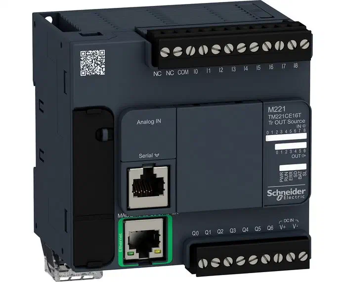
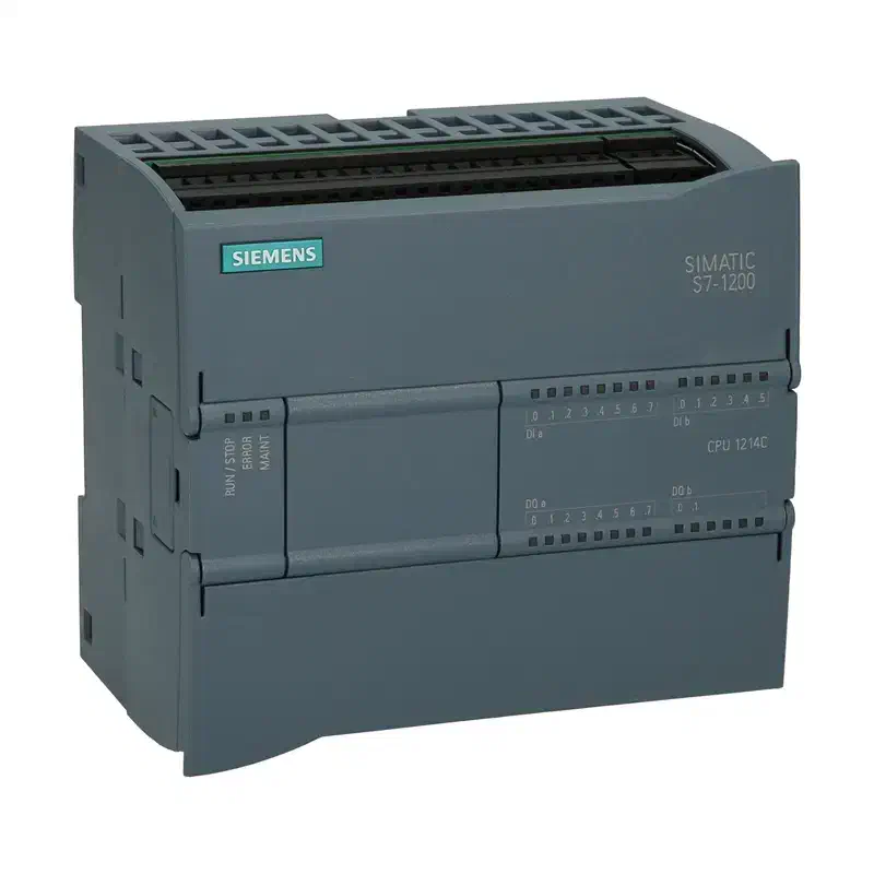
Why not use a standard PC?
A PC cannot guarantee deterministic execution: it can freeze, reboot, or delay critical tasks due to background processes or OS-level interrupts. In control systems, this leads to a catastrophic loss of control over the physical process.
A PLC, unlike a PC, is built for deterministic and resilient operation:
- It executes logic sequentially in a strict, cyclic loop (Scan Cycle);
- It guarantees deterministic processing of inputs and outputs;
- It utilizes hardware-level fail-safes (e.g., Watchdog timers).
It is important to note that PLCs are also subject to system interrupts, which can cause undesirable artifacts – such as timer and oscillator clock drift – but this will be covered in future articles.
PLC Operation Principle:
- Read input statuses;
- Execute programmed logic;
- Update output states.
This cycle repeats continuously with microsecond precision.
The pendant buttons are wired to the PLC’s inputs, while its outputs drive the contactor’s coil circuit (typically routed through intermediate elements like safety relays).
Detailed PLC hardware configurations and output topologies (Transistor vs. Relay) are discussed below.
PLC Configurations: Transistors, Relays, and Inputs
PLCs are available in several hardware configurations, for instance:
24 V DC / DC / DC (Solid-State Transistor Outputs)
- 24 V DC (Power): The PLC requires an external 24 V DC power supply;
- DC (Inputs): Digital inputs are designed for 24 V DC signals (e.g., from sensors or switches);
- DC (Outputs): Digital outputs utilize solid-state transistors to commutate 24 V DC;
- Transistors are exceptionally fast, silent, and have a near-infinite mechanical lifespan;
- DC only; commutating heavy AC loads requires an external relay or contactor.
220 V AC / DC / Relay (Relay Outputs)
- 220 V AC (Power): The PLC runs on 220 V AC mains power, meaning it plugs directly into the grid;
- DC (Inputs): Digital inputs read 24 V DC signals;
- Relay (Outputs): Mechanical relays actuate the outputs, capable of switching both AC and DC;
- High versatility (AC/DC);
- Relays are slow, suffer from mechanical contact wear, and are extremely difficult (or impossible) to service without replacing the PLC.
There are also 24 V DC / DC / Relay variants.
The core advantage of solid-state transistors over relays is the absolute lack of moving parts. Switching occurs at the semiconductor crystal level (PN junction), therefore:
- A transistor suffers zero mechanical wear, generates no sparks, and can endure virtually limitless switching cycles provided no dielectric breakdown occurs;
- Conversely, a mechanical relay’s lifespan is physically limited to hundreds of thousands or a few million cycles.
Furthermore, transistors operate at vastly superior switching frequencies:
- Transistor turn-on/turn-off times are measured in microseconds to tens of microseconds (µs). They can switch at frequencies up to several kHz (sometimes tens of kHz);
- Relay actuation takes 5–20 ms (sometimes more). The maximum switching frequency is bottlenecked at 5–10 Hz.
Relay outputs in a PLC are usually soldered directly to the PCB. If a relay contact fuses, the entire PLC must be replaced.
A topology utilizing a solid-state PLC output driving an external contactor is vastly superior and cheaper to maintain. If the contactor fails, it is simply swapped out as a modular unit – a process magnitudes faster and cheaper than replacing a highly configured PLC.
For our use case, the optimal hardware is 24 V DC/DC/DC, because the actual load switching will be handled by a rugged contactor, whose coil we will drive via the PLC’s transistor output (routed through a safety relay and protected by a flyback diode, detailed later).
2.3. E-STOP and Safety Relays
In strict compliance with ISO 13850 (Emergency stop function) and ISO 13849-1 (Safety-related parts of control systems), the architecture must follow the Fail-Safe principle. This is precisely why NC (Normally Closed) contacts are mandatory: if a wire snaps or a forklift rips the pendant off the wall, the current flow ceases, and the system instantly enters a fail-safe state (trips).
If NO (Normally Open) contacts were used, a severed wire would silently disable our ability to halt the machinery.
The mandate for dual-channel redundancy (2 NC contacts) routed through a dedicated safety relay elevates our node to Safety Category 3 (Performance Level ’d’) – meaning the system retains its safety function even in the event of a single point of failure (e.g., if one of the button contacts structurally welds closed).
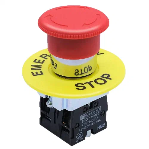
It is critical to note that the market is flooded with cheap E-Stop buttons utilizing a single 1NC contact, but we strictly require a 2NC block, alongside a certified safety relay.
A safety relay (referencing the Intermediate Relay class) is a specialized safety logic device spliced into the control circuit – in our architecture, sitting directly between the PLC’s transistor output and the contactor coil:
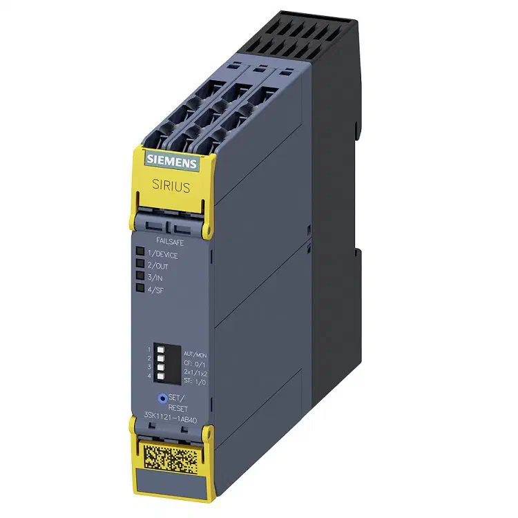
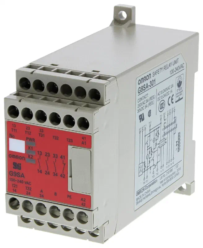
The safety relay continuously monitors the dual-channel loop of the E-Stop button. The moment a discrepancy is detected (either contact opens), it mercilessly severs the control signal circuit, locking the system in a tripped, fail-safe state until a deliberate reset signal is asserted.
Resets can be automatic or manual; we will dissect this later.
2.4. Control Panel
We will also procure:
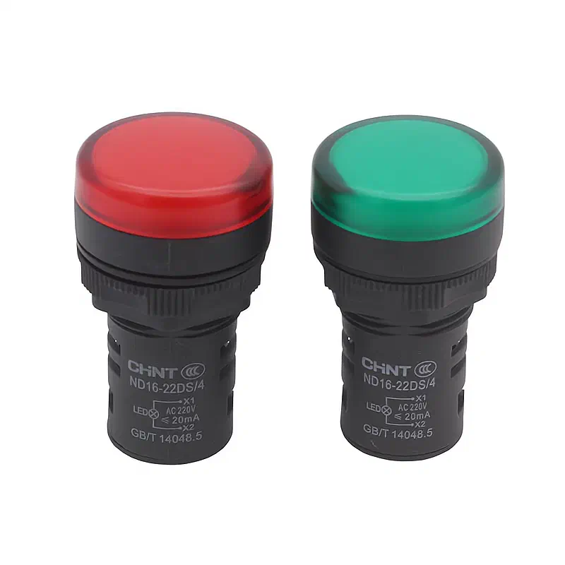
- 220 V indicator lights (with DIN-rail mounting adapters) for voltage presence monitoring;
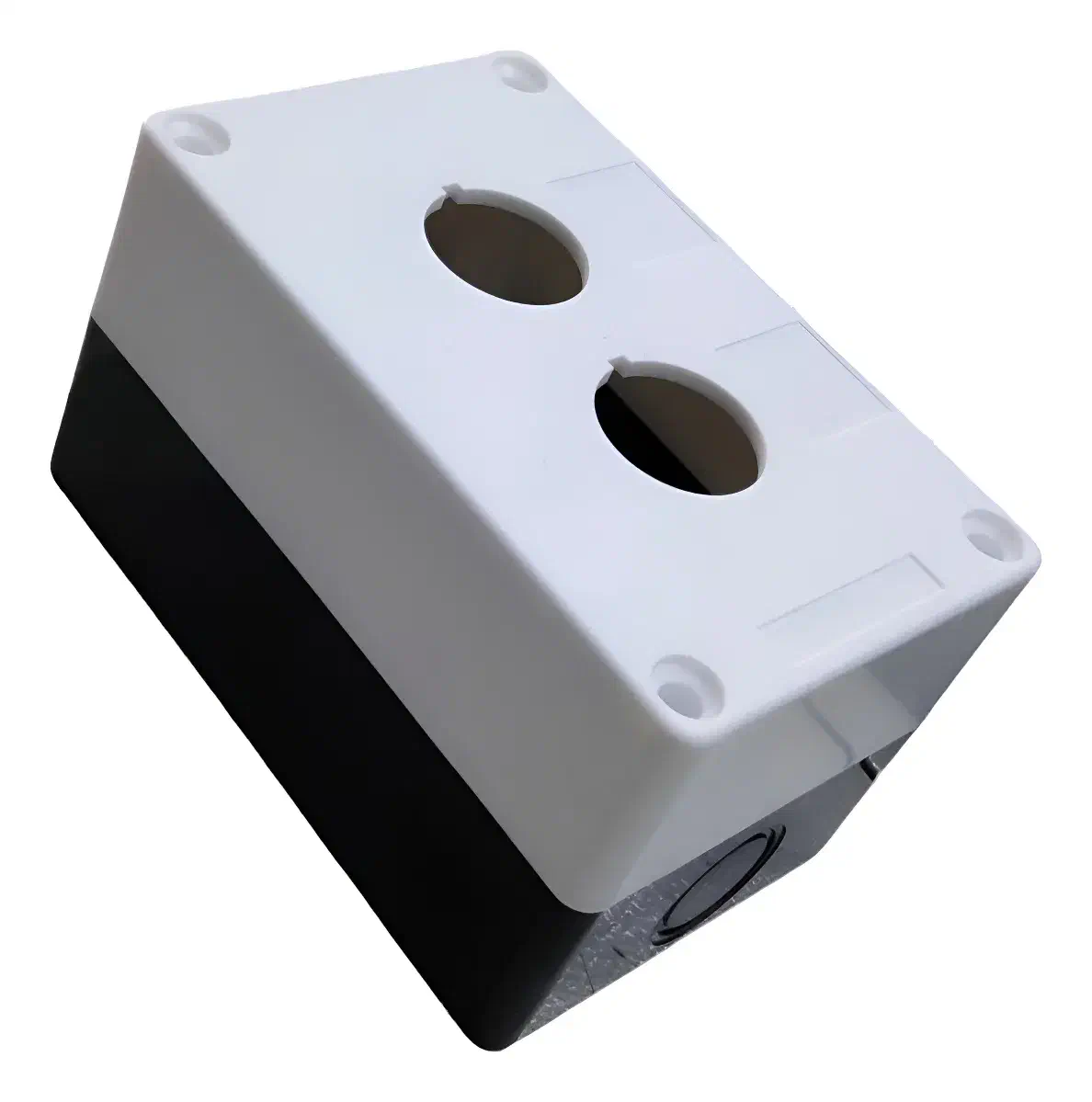
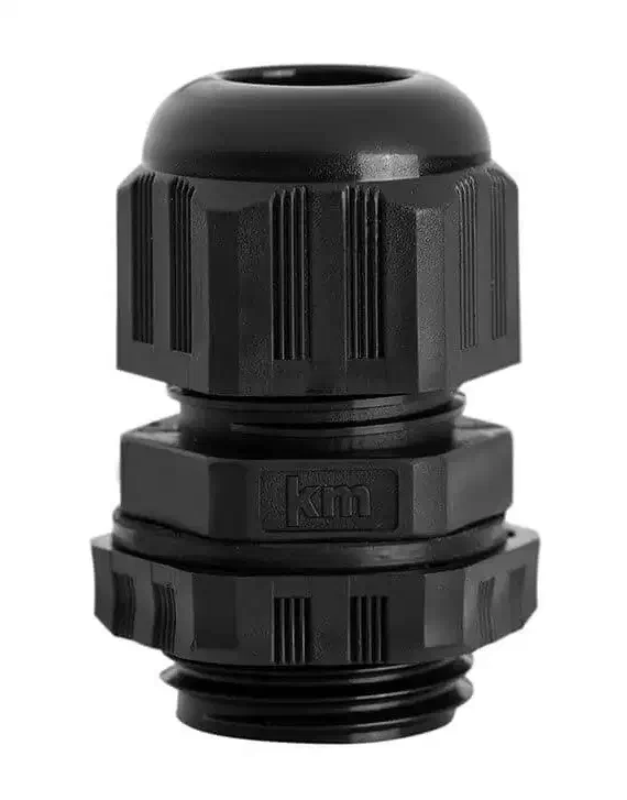
- A pushbutton enclosure (station) for Ø22 mm switches, equipped with a cable gland;
- Ø22 mm pushbuttons (Start/Stop); remembering that the START button must be NO (Normally Open), while the STOP button must be NC (Normally Closed);
- A DIN-rail mounted power socket to serve as our physical load simulator.
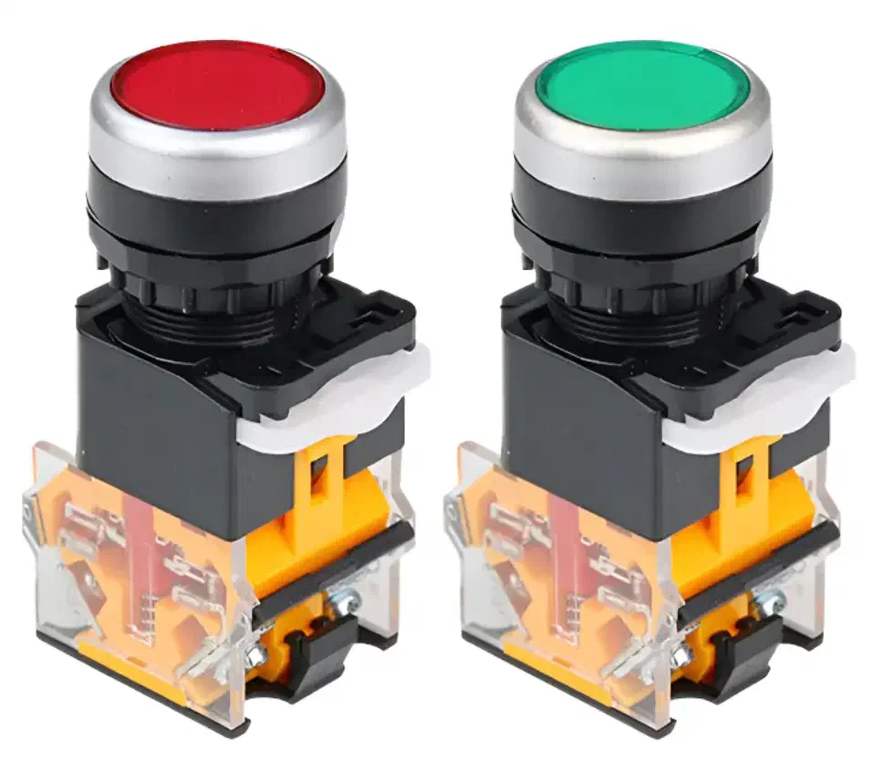

2.5. Power Supply
A DIN-rail Power Supply Unit (PSU) is required to rectify 220 V AC mains into 24 V DC to energize the PLC and control circuits, including the safety relay:
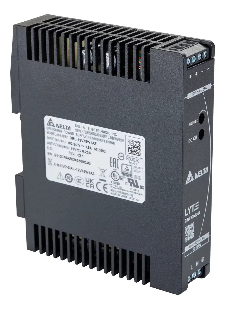
Note: There is a critical engineering caveat regarding undervoltage protection logic, which we will analyze later.
Furthermore, short-circuit and overcurrent protection must be strategically tiered:
- Main input circuit breaker;
- Dedicated circuit breaker for the power circuit (load);
- Dedicated circuit breaker for the PSU primary (“Input”);
- Fused distribution for 24 V DC bus segments (“Output”).
Note: There are critical nuances regarding Time-Current Characteristic (TCC) curves, which we will dissect further down the line.
We also require a single-phase energy meter featuring a built-in voltmeter, ammeter, and frequency counter, equipped with Modbus telemetric polling via an RS-485 bus:
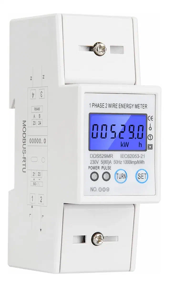
When selecting components, you must verify that the chosen PLC model natively supports Modbus communication; if not, an RS-485 expansion module (communication board) must be procured.
Modbus RTU is an Application Layer protocol (OSI Layer 7) that dictates the logical structure of the message payload.
RS-485 is the Physical Layer standard (OSI Layer 1). Data is transmitted electrically via differential signaling (measuring the potential difference between twisted pair wires A and B).
3. System Design
During the design phase, we must resolve two critical tasks:
- Control Cabinet Layout (spatial positioning of components);
- Wiring Diagram (electrical schematics / drawings).
If a highly detailed layout analysis is required, enterprise software like EPLAN can be utilized. However, for our objectives, a lightweight open-source solution is perfectly adequate: QElectroTech.
3.1. Cabinet Layout
A layout sheet in QElectroTech is referred to as a “Folio”. By default, the folio is named Untitled.
Right-click on it → Folio Properties → Title → change to Cabinet layout.
Components in an ICS control cabinet (as well as standard electrical panels) are mounted on a DIN-rail:
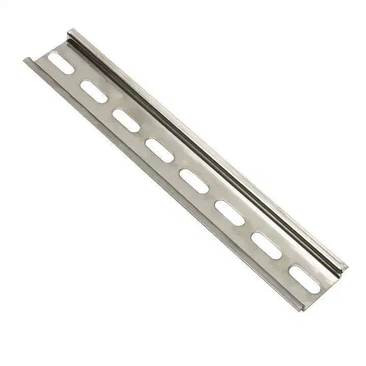
In QElectroTech, select the rectangle tool and schematically draw a DIN-rail:
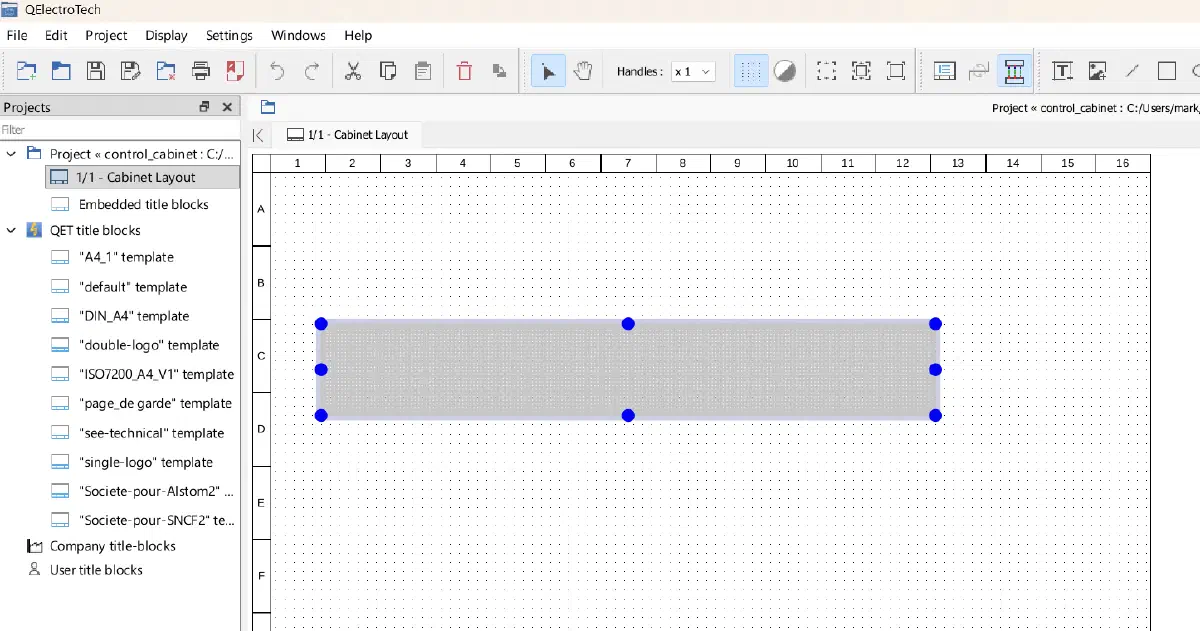
Pro Tip: If you need to resize the drawn rectangle – clicking the default frame (green markers) scales the element symmetrically, which is inconvenient. Double-clicking the frame reveals blue markers, allowing independent manipulation of each side.
We have already established that the power circuit is physically segregated from the control circuit. Our testbed will feature three tiers:
- Grid input, power circuit, 220 V AC;
- Control loop, 24 V DC;
- Operator panel / remote control pendant.
Next, resize the folio → double-click the frame → set Columns = 13 and Rows = 15. Following this, draw three parallel DIN-rails:
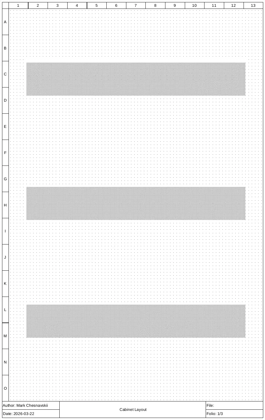
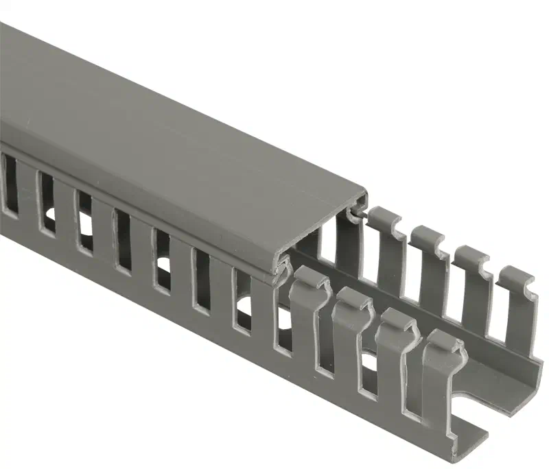
In industrial automation cabinets, all cables are routed through slotted cable ducts (wireways) forming a closed perimeter.
The baseline form factors for cable ducts are 25x25 mm and 25x40 mm (first and second photos, respectively), though numerous variants exist.
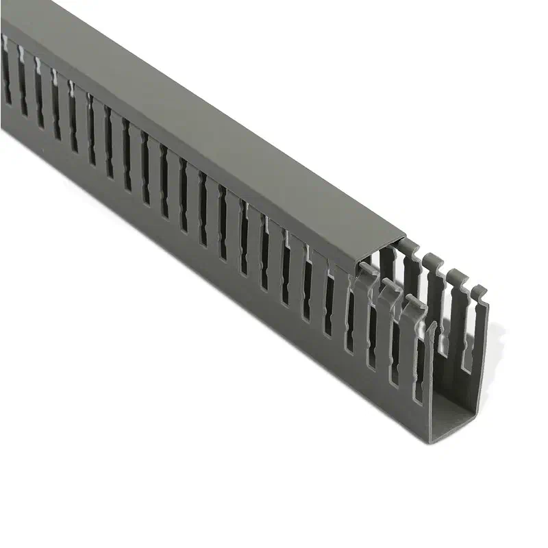
Returning to QElectroTech, mark the cable ducts along the perimeter and between the tiers:
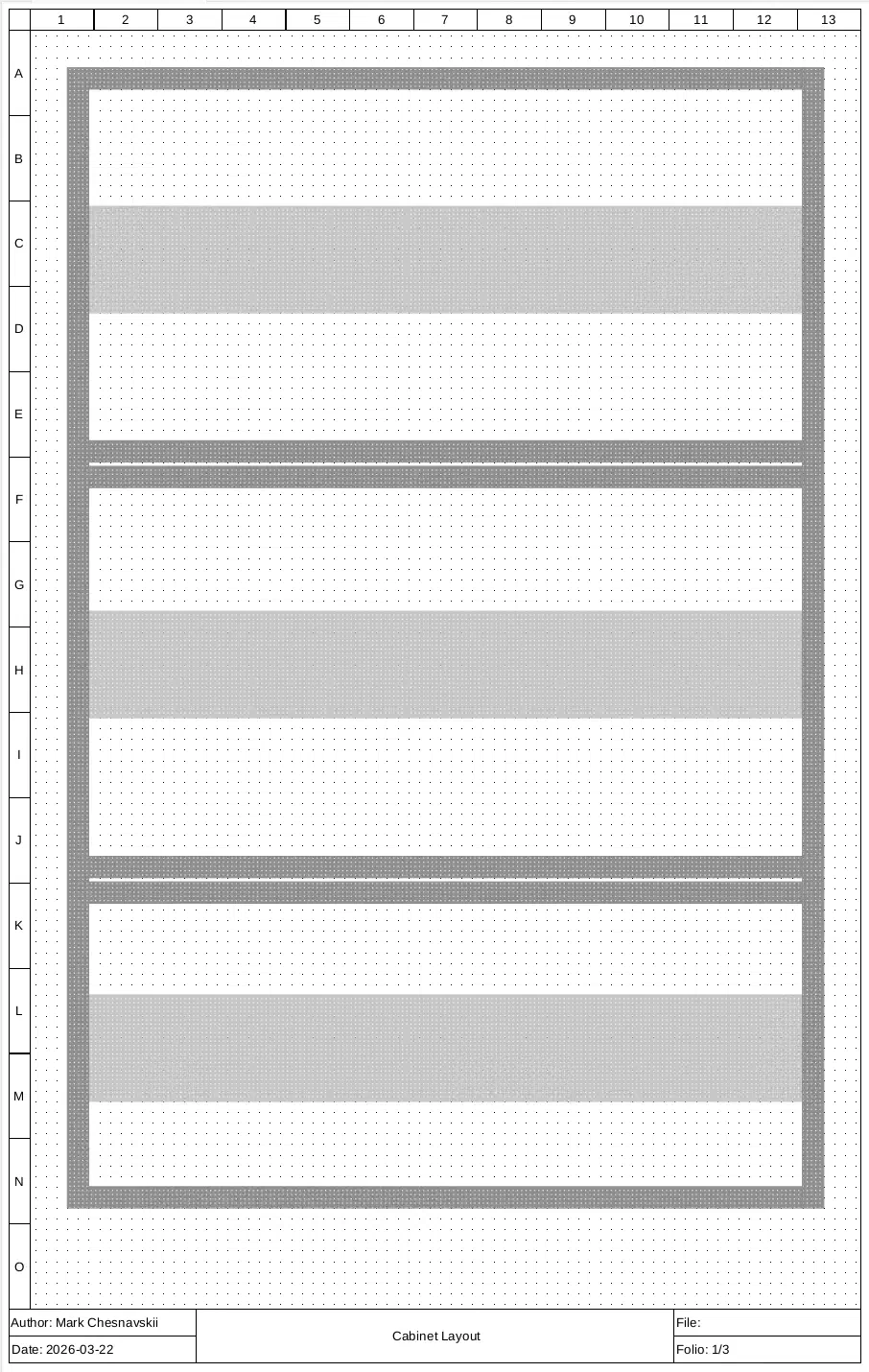
Note the dual cable ducts between the tiers. This design choice is mandatory to mitigate EMI (Electromagnetic Interference) induced by high-voltage power cables onto the low-voltage control signals and the RS-485 bus: one duct is strictly for power lines, the other for control signals and telemetry.
Crossing these lines is permissible only at a strict 90-degree right angle.
On the right side of the software interface, locate the “Collections” panel:
QET Collection → Electric → Graphics: We will use this section for the physical layout;QET Collection → Electric → All pole: This is required for the wiring diagram (schematics);User Collection: A critical section detailed below.

Any element in QElectroTech can be customized as follows:
- Right-click the element;
- Select “Edit element”;
- In the element editor, go to File → Save as;
- Duplicate/save the modified copy into the User Collection.
Personal Component Library and Collections Backup
You can duplicate existing elements, save modified copies, or draft entirely custom elements from scratch.
This is highly efficient and, in many cases, mandatory to keep all frequently used components readily accessible. Feed-through terminal blocks, distribution bars, power supplies, contactors, pushbuttons, etc.
Critical: For a new or modified element to appear in the “Collections” panel, right-click the respective section → select “Reload collections”.
Furthermore, it is standard practice to back up your custom element collection: right-click the section → “Open the underlying folder”. Then securely copy this directory to backup storage.
Next, we populate the 220 V AC power tier.
Assuming the facility’s main distribution board utilizes a C20 circuit breaker, we select the following MCB (Miniature Circuit Breaker) ratings:
- C10: Main input breaker for the testbed;
- C6: Dedicated load breaker * (nuances apply here);
- C6: Dedicated PSU (AC 220 V → DC 24 V) breaker * (nuances apply here).
It is necessary to clarify the classes of circuit breakers:
- MCB (Miniature Circuit Breaker) – up to ~100 A, overload and short-circuit protection;
- MCCB (Molded Case Circuit Breaker) – heavy-duty, up to hundreds of amperes;
- ACB (Air Circuit Breaker) – massive, for industrial-grade mains distribution.
We are operating with MCBs.
Below, we dissect the engineering physics behind circuit breaker selection.
01. Core Principles
A circuit breaker is defined by the following parameters:
- Time-Current Characteristic (TCC) curve (trip “speed”);
- Nominal Current ($I_n$);
- Protection functions (Trip unit types: thermal and/or magnetic);
- Number of poles.
The breaker must unconditionally satisfy the primary rule of cable line protection.
Thereafter, the selection becomes a calculated compromise between two states:
- Short-circuit selectivity;
- Overload selectivity.
Selectivity (Coordination) is the protection system’s ability to isolate strictly the faulted segment of the circuit without tripping the entire facility upstream.
02. Cable Line Protection
The paramount rule for cable line protection is: $$ I_b \leq I_n \leq I_z $$
Where:
- $I_b$ – Design current (operational load current);
- $I_n$ – Nominal rating of the circuit breaker;
- $I_z$ – Continuous current-carrying capacity of the cable (dictated by cross-section, material, and routing conditions).
Power Circuit:
According to project requirements, the load current $I_b$ = 5 A; the selected C6 breaker: $I_n$ = 6 A. The power cable we will utilize (1.5 mm²) has an $I_z \approx$ 15-18 A.
Validating the condition: $$ 5 \text{ A} \leq 6 \text{ A} \leq 16 \text{ A} $$
Control Circuit (PLC, Relays):
We finalize a 75 W Power Supply Unit (PSU). In steady-state operation, its current draw from the 220 V grid (inrush current will be addressed shortly) is: $$ I_b \approx P/V \approx \frac{75}{220} = 0.34 \text{ A} $$
Thus, the steady-state load current $I_b$ = 1 A (with margin); the selected C6 breaker: $I_n$ = 6 A. The control cable we will utilize (1.0 mm²) has an $I_z \approx$ 10-12 A.
Validating the condition: $$ 1 \text{ A} \leq 6 \text{ A} \leq 11 \text{ A} $$
03. Number of Poles
Circuit breakers are classified by poles:
- 1P (Single-pole) – interrupts one conductor (usually phase);
- 2P (Double-pole) – interrupts both phase and neutral;
- 3P (Three-pole) – for three-phase grids (three phases);
- 4P – three phases + neutral.
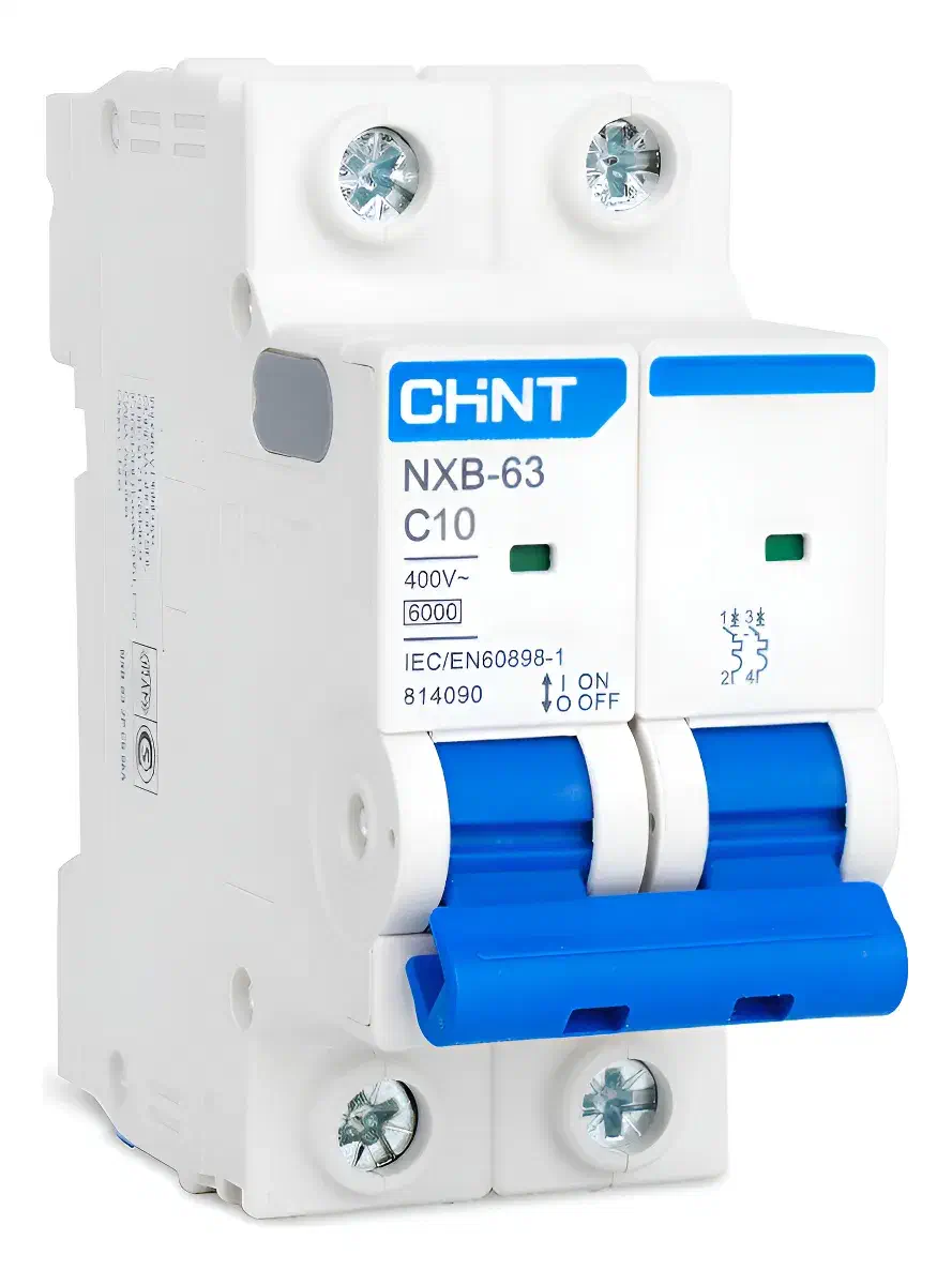
For our testbed, we mandate 2P (Double-pole) breakers.
Reviewing the CHINT NXB-63 lineup:
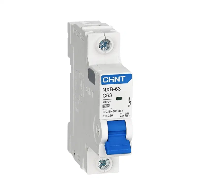
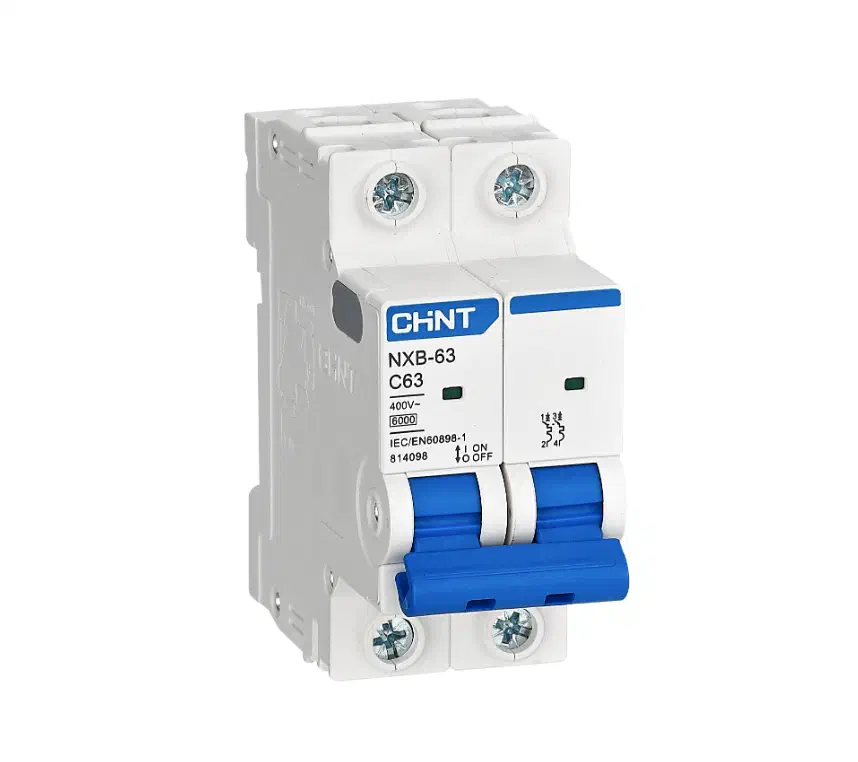
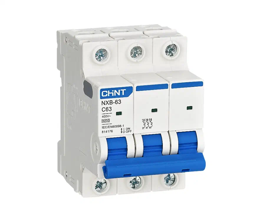
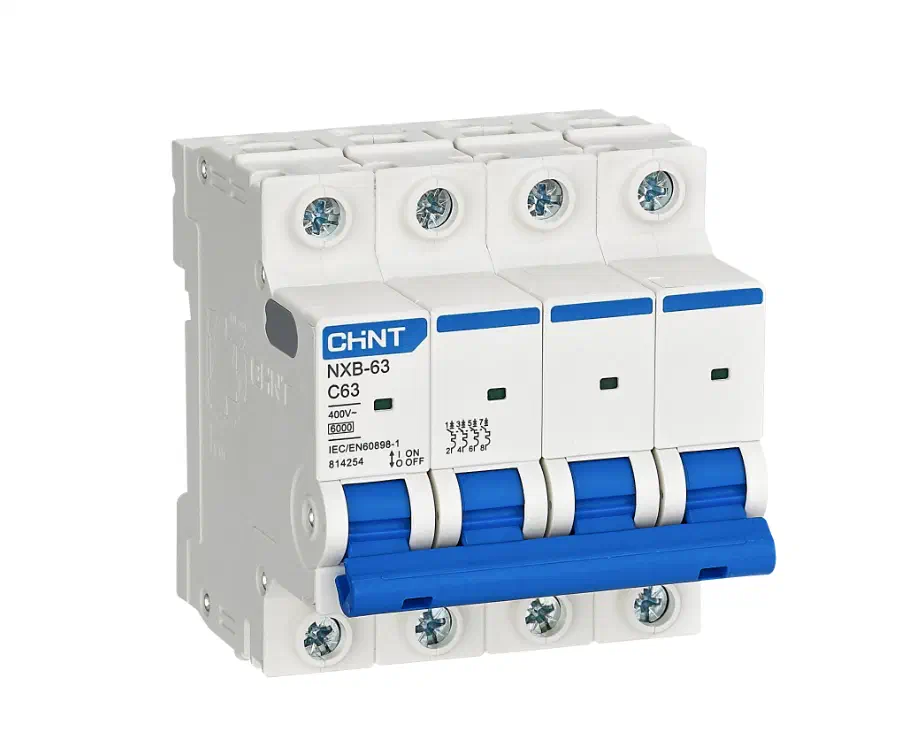
04. Protection Types and Trip Units
It is critical to verify the protection type embedded within each pole.
There are two fundamental protection mechanisms:
- Overload protection (Thermal release);
- Short-circuit protection (Magnetic release).
Reviewing the schematic symbols:
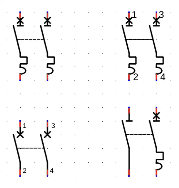
Symbology Breakdown:
Dashed line (between contacts):
- Mechanical linkage. Indicates the poles are interlocked: if one trips, it forces the other to open.
- They are actuated simultaneously via a single toggle.
Cross (X) on the upper contact:
- Automatic disconnection capability. The defining trait of a breaker (presence of an arc chute). This is a
- heavy-duty mechanism capable of safely rupturing massive fault currents.
Horizontal bar (T-shape top) on the contact:
- Switch-disconnector (Isolator). A contact devoid of protection logic. Functions purely as a manual ON/OFF switch.
Square step (U-shaped protrusion at the bottom):
- Magnetic release. The short-circuit sensor. Triggers an instantaneous trip command upon detecting a severe current spike.
Semicircle (arc at the bottom):
- Thermal release. The overload sensor (bimetallic strip). Triggers a trip command if the current moderately exceeds the threshold for a sustained duration (protecting wiring from thermal degradation).
Carefully examining the symbol printed on one of the CHINT breakers:
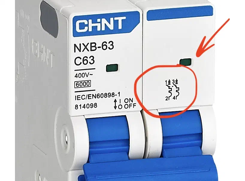
Observation reveals that each pole is equipped with both a thermal release (overload) and a magnetic release (short circuit).
05. Overload Selectivity
Selectivity for each trip mechanism (thermal for overload and magnetic for SC) must be calculated independently.
Calculating overload selectivity.
Tripping formula: the higher the current exceeds $I_n$, the faster the breaker trips.
Our breaker chain: C20 (Facility) → C10 (Testbed Input) → C6 (Internal Segment).
If an inductive load stalls and begins drawing 8 A:
- The C6 breaker registers this (~30% overload), heats up, and trips;
- The C10 breaker, experiencing 8 A, continues uninterrupted operation (current is below its nominal rating).
For overloads (currents exceeding operational parameters but short of a dead fault), selectivity in our topology is 100% absolute.
06. PSU Inrush Current
A critical, often overlooked physical trait of Switch-Mode Power Supplies (SMPS):
Inside an SMPS, immediately following the diode bridge rectifier, sit massive, discharged bulk capacitors.
The moment AC voltage is applied, these capacitors draw a violent, instantaneous surge of current to charge – an Inrush Current lasting merely a few milliseconds.
Consult the datasheet for our PSU, DRL-24V75W1AZ:
https://psu.deltaww.com/en/products/configurable-power-supply/DRL-24V75W1AZ
Navigate to the link above → locate the “Download” section → “Datasheet”:
https://psu.deltaww.com/en/products/download/Datasheet/DRL-24V75W1AZ
Locate the “Max Inrush Current” metric:
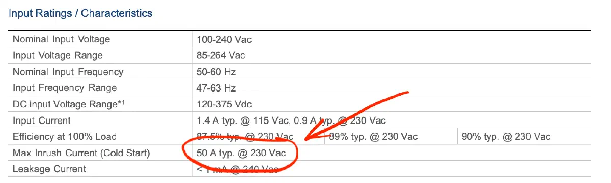
Conclusion: Despite the 75 W PSU’s steady-state operating current not exceeding 0.5 A, the instantaneous inrush current during a cold start at 230 V can violently spike to 50+ Amperes!
Incidentally, this current transient can be captured physically using an oscilloscope paired with a Hall-effect current probe. We will conduct this hardware-level analysis in upcoming articles.
07. Why are bulk capacitors required in a PSU?
The PSU converts 220 V AC into 24 V DC.
In highly simplified terms, an SMPS topology is:
- Rectification of input 220 V AC to 311 V DC (recall that 220 V is an RMS value);
- A PWM controller and a switching MOSFET chopping this DC at tens/hundreds of kHz – yielding a high-frequency “pulsed” 311 V;
- A high-frequency transformer stepping the 311 V down to 24 V AC (surprise!);
- Secondary rectification from 24 V AC to 24 V DC (yes, again!).
At high frequencies, the transformer generates significantly less heat and requires a fraction of the copper windings. This entire complex topology exists purely to manufacture highly compact PSUs with maximum efficiency.
Our focus is the primary input rectifier. This consists of a diode bridge + a filter capacitor on its output.
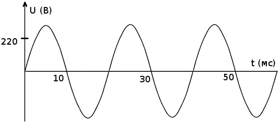
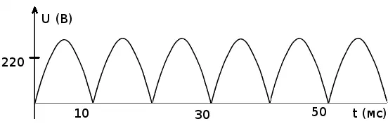
The bridge takes the sine wave → full-wave rectification. The ripple frequency doubles, and the waveform becomes a series of absolute-value pulses ($|sin|$).
The AC voltage at the input of the diode bridge looks like this (50 Hz, meaning period $T=\frac{1}{f}=\frac{1}{50}=0.02$ sec, half-period is 10 ms):
At the output of the diode bridge:
The capacitor charges to the absolute peak (~311 V, since 220 V is merely the RMS value) and then discharges between peaks, sustaining the voltage level and smoothing the ripples:
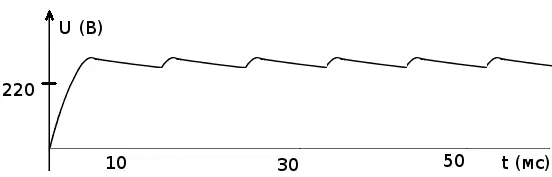
Smoothing is the primary function of the capacitor. However, it provides a critical secondary effect: during transient input voltage sags (brownouts lasting milliseconds), the PSU can maintain a stable 24 V DC output utilizing the stored energy.
This parameter is known as Hold-up Time, and it is explicitly listed in the datasheet. This is mission-critical when powering digital logic like PLCs or safety relays.
Furthermore, leveraging the Hold-up Time specification, we can reverse-engineer the approximate capacitance.
Knowing the input voltage and the capacitance, we can mathematically deduce what the true, destructive inrush current would be – if the manufacturer had omitted rudimentary protection circuitry.
08. Inrush Current Mitigation Strategies
Here we analyze the problem from the perspective of an SMPS manufacturer.
Option 1. Series Resistor
Primitive and inefficient:
- Limits current, but constantly dissipates massive thermal energy (Joule heating) since it is permanently inline;
- Viable only for very low-power units (< ~30 W).
Option 2. NTC Thermistor (Negative Temperature Coefficient)
The industry standard:
- Cold state → high resistance → chokes the inrush current;
- Heated state → resistance plummets → allows normal operation.
Drawbacks:
- Highly temperature-dependent;
- Fails utterly during rapid power cycling (hot starts, as the thermistor hasn’t cooled down).
Option 3. Resistor + Solid-State/Relay Bypass
A superior engineering topology:
- At startup → current flows through the resistor;
- Post-startup → a relay/MOSFET shunts (bypasses) the resistor.
Advantages:
- Zero parasitic losses during steady-state operation;
- Thermally stable;
- Immune to rapid power cycling issues.
Option 4. Active Current Control (Soft-Start via MOSFET)
The cutting-edge approach:
- Active current limitation (soft-start logic);
- No discrete resistor (the switching MOSFET itself operates in the linear region to throttle current).
Advantages:
- Maximum efficiency;
- Minimal PCB footprint;
- Independent of input grid fluctuations.
09. How does our PSU mitigate inrush current?
Inrush current is a function of voltage and capacitance. Let’s assume a 230 V grid.
The capacitor charges to the amplitude (peak) voltage. For 220-230 V RMS, the peak is $V_{peak}=V_{rms} \cdot \sqrt2 \approx 311..325\ \text{V}$.
We will use 325 V for our calculations.
How do we deduce the bulk capacitance? It is conspicuously absent from the datasheet.
The trick is to reverse-engineer it using the “Hold-up Time” parameter discussed earlier:
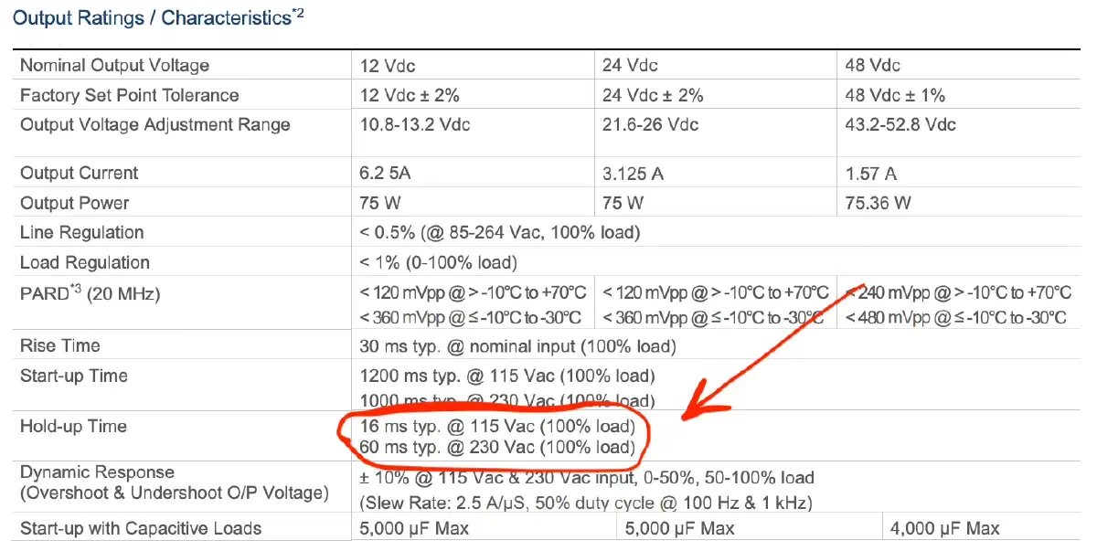
Datasheet value: 60 ms at 230 V.
Energy stored in a capacitor: $$ E=\frac{1}{2}CV^2 $$
It is critical to note that the PSU’s PWM controller shutting down (Undervoltage Lockout) occurs when the capacitor voltage decays to roughly 100-120 V DC.
Thus, the PSU does not drain the capacitor to absolute zero, but rather from 325 V down to ~100 V. Therefore, the precise energy equation sustaining the PSU during hold-up is:
$$ \Delta E=\frac{1}{2}C(V_{max}^2-V_{min}^2) $$
Output power: $$ P=75 \text{ W} $$
However, to deliver 75 W, the PSU draws more power from the capacitor due to switching losses, thermal dissipation, etc. – efficiency is never 100%.
A standard industrial SMPS efficiency is approximately 88-90%: $$ \eta=\frac{P_{out}}{P_{in}} $$
Thus, the actual power drained from the capacitor: $$ P_{in}=\frac{P_{out}}{\eta}=\frac{75}{0.89} \approx 84.3\ \text{W} $$
Consequently, the energy required for 60 ms of Hold-up Time is: $$ E=P \cdot t = 84.3 \text{ W} * 0.06 \text{ sec} \approx 5.06 \text { J} $$
Substituting: $$ 5.06=\frac{1}{2}C(325^2-100^2) $$
$$ 10.12=C(105625-10000) $$
Capacitance: $$ C=0.00010583=105.83 * 10^{-6}\ \text {F}=105.83\ \text{µF} $$
In our DRL-24V75W1AZ power supply, it is highly probable that the manufacturer utilized an NTC thermistor alongside a
bulk capacitor rated at roughly 120-150 µF. Manufacturers always over-provision capacitance to account for electrolytic
degradation over time (usually +20-40% above the theoretical minimum).
For safety margins, we assume a 150 µF capacitance.
Could we map the exact function of the raw inrush current lacking an NTC thermistor? $$ I_{inrush}(t)=\frac{V_{peak}}{R_{total}} \cdot e^{-\frac{t}{RC}}\ \text{A} $$
Where:
- $V_{peak} \approx 325\ \text{V}$
- $R_{total}$: The aggregate series impedance (wiring + bridge + Equivalent Series Resistance (ESR) of the capacitor). Unprotected, this is $\approx 1–3\ \Omega$.
And then map the current with an NTC, calculating the exact amperage at 1 ms, 5 ms, and 10 ms, to compare it against a C2 or C4 breaker’s instantaneous trip threshold?
We wish!
The critical flaw is that this formula assumes a perfect DC circuit. We are feeding it $|\sin|$ pulses from a diode bridge. The capacitor does not charge in a smooth, continuous monotonic curve as it would under pure DC; it charges in violent micro-bursts, only during the exact milliseconds when the instantaneous $|\sin|$ voltage exceeds the capacitor’s current voltage level!
This results in a series of aggressive, needle-like spikes. The first spike is the widest and most destructive (since the capacitor is initially at 0 V). This is the source of the 50 A transient listed in the datasheet.
We will verify this empirically on an oscilloscope later.
The PSU datasheet provides this graph:
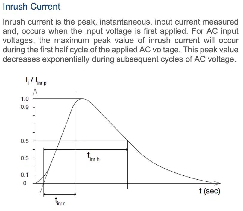
Furthermore, an NTC thermistor cannot be modeled as a static resistor – that is its exact feature. Its resistance decays as it heats, meaning the true dynamic inrush current at specific intervals would exceed theoretical static calculations.
It is critical to state that the NTC thermistor – installed to prevent the PSU from drawing absolutely catastrophic currents (which could hit 100…300 A in the first millisecond!) – inherently increases the capacitor’s charging time ($t_{inrush}$)!
Delta (the manufacturer) mitigates the peak amplitude of the surge but pays the price in an extended $t_{inrush}$ duration.
Physics dictates: the thermistor chokes the current → the capacitor requires more time to hit peak voltage. Furthermore, as established, it charges in discrete bursts, not continuously.
The exact $t_{inrush}$ value is not explicitly written, but it is the point on the graph where $t_{inrush}$ drops to $\approx$ 0 A. That duration stretched significantly when Delta integrated NTC protection.
Therefore, we cannot mathematically predict the exact real-time behavior of the inrush current over the first 10 ms. We are bound to the datasheet empirical limits.
The raw math (lower limits):
- A C2 breaker would trip at 10 A (5 * 2 A) at 10 ms;
- A C4 breaker would trip at 20 A (5 * 4 A) at 10 ms.
Given that an NTC’s resistance drops when hot, rapid power cycling could easily trip a C2 or C4. For guaranteed stability, a C6 is the pragmatic engineering choice.
We will analyze breaker TCC curves in the next section.
10. Short Circuit Selectivity
Recall that circuit breakers are defined by their Time-Current Characteristic (TCC) curve.
The standard industry curves:
- Curve B: Trips at ~3–5× nominal current (Highly sensitive, for resistive loads);
- Curve C: Trips at ~5–10× (Universal, the baseline standard);
- Curve D: Trips at ~10–20× (For massive inrush currents: motors, heavy transformers).
Specialized curves:
- Curve K: For highly inductive loads;
- Curve Z: Ultra-sensitive (solid-state electronics protection).
For our load, Curve C is technically appropriate, but the reality is complex. A Curve C magnetic release trips between 10-100 ms at currents ranging from $5 \cdot I_n$ to $10 \cdot I_n$.
Let’s review our breaker topology:
- C20: Facility main;
- C10: Testbed main input;
- C6: Load branch;
- C6: PSU branch.
Calculating instantaneous trip thresholds:
- C6: Trips between 30 A and 60 A;
- C10: Trips between 50 A and 100 A;
- C20: Trips between 100 A and 200 A.
What happens during a dead (hard) short circuit (e.g., phase shorted to neutral on the output of the C6)?
A hard short-circuit fault current ($I_{sc}$) in a standard facility ranges from 200 A to 800 A (depending on the transformer distance/loop impedance). Assume $I_{sc}$ = 300 A. This devastating current instantly propagates through the entire chain: C6, C10, and C20.
Since 300 A massively exceeds the trip threshold of all breakers in the chain (even the C20 maxes out at 200 A), they will all attempt to trip simultaneously. Practically, whichever mechanism physically separates its contacts first wins.
There is a high probability that a short on our testbed will trip the main facility breaker (C20).
Conclusion: Cascading modular MCBs of the same curve in series does not guarantee short-circuit selectivity. A fault current massively exceeding the magnetic threshold of upstream breakers will trigger an unpredictable, sympathetic (cascading) trip.
The theoretically perfect solution: Curve D on the facility main, Curve C at the testbed input, Curve B on internal branches.
Why can’t we install a B6 on the load or PSU? Because Curve B is explicitly for resistive loads with zero inrush. The PSU inrush or inductive kick would instantly trigger nuisance tripping.
We face an engineering paradox: we need a “fast” breaker for SC selectivity (Curve B) but a “slow” breaker to survive PSU inrush and inductive transients (Curve D).
This is a classic control cabinet design dilemma. Curve C became the ubiquitous industrial and domestic standard exactly because it serves as the optimal compromise between fault protection and transient immunity.
In real-world OT environments, operational stability is heavily influenced by power quality. A highly critical threat vector is undervoltage (brownouts), caused by grid sags, massive motor startups, or degraded power infrastructure.
In such states, digital equipment behaves erratically: PSUs trip, PLCs undergo unexpected resets, and actuators fire randomly.
In industrial practice, undervoltage protection is implemented via a two-tier architecture:
- On the primary grid side, a dedicated Voltage Monitoring Relay (and Phase Failure relay for 3-phase) is deployed. If parameters breach safe thresholds, it hardware-interlocks the control logic.
- On the control loop side, the PSU’s “DC OK” dry contact signal is monitored. If it drops, the control circuit is deliberately broken, de-energizing contactors and forcing the system into a fail-safe state.
Directly cutting power to a 24 V DC bus due to undervoltage is bad practice. Instead, controlled shutdown logic is enforced (via the “DC OK” signal), preventing undefined PLC states and ensuring predictable process degradation.
Our specific Delta DRL-V75W1AZ PSU relies entirely on LED indication for “DC OK” and lacks a discrete dry-contact
output.
The 220 V AC tier layout is sequenced left to right:
- Feed-through terminal blocks for main input: Phase, Neutral, and Ground (PE, bonded to the DIN-rail);
- Main input MCB
CHINT NXB-63 C10 2P; - Power distribution blocks for Phase and Neutral;
- Grid voltage presence indicator
CHINT ND16-22DS/4; - Load MCB
CHINT NXB-63 C6 2P; - Modbus (RS-485) energy meter for load monitoring
SinoTimer DDS529MR; - PSU MCB
CHINT NXB-63 C6 2P; - Switch-Mode Power Supply
Delta DRL-V75W1AZ 75W; - Dedicated DIN-rail ground terminal block for the PSU.
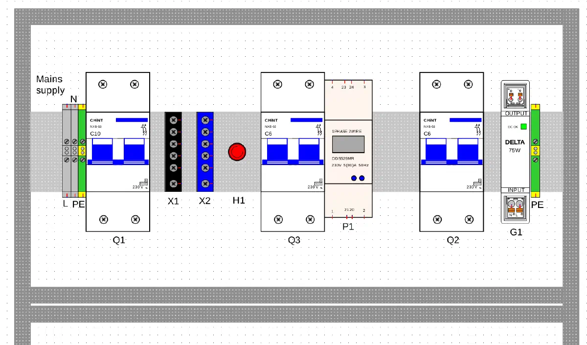
Now we lay out the 24 V DC (PELV) control tier.
It is critical to note that every distinct control loop (PLC, relays, control pendant) will be protected by its own dedicated fuse, achieving strict bus segmentation.
This exact topology is standard in automotive engineering – every segment of the 12 V bus is independently fused.
Fuse ratings:
- 1 A for PLC main power;
- 2 A for PLC output logic power (outputs are powered on a separate rail!);
- 1 A for the control pendant;
- 1 A for the safety relay.
Why use fuses on a 24 V DC bus?
Why add fuses to the 24 V line if we already have a C6 breaker upstream of the PSU?
The core issue lies in galvanic isolation.
Recall the architecture of an SMPS – it utilizes an isolation transformer. By physical definition, the 24 V DC output is completely isolated from the 220 V AC input.
If a dead short occurs somewhere on the 24 V loop, the upstream C6 breaker is completely blind to it.
How does the PSU react? An interesting physical mechanism occurs. Upon detecting a dead short on its output, the PSU drops into “Hiccup mode”: attempt startup → detect short → shutdown → wait → re-attempt.
Why not just rely on the PSU’s internal protection? Because during a localized short circuit, the entire automation node will repeatedly reboot until the fault is cleared. This is an unacceptably blunt response.
Fuses are sacrificial components. A short on the control loop could simply be a crushed wire at the remote operator pendant.
This is precisely why the 24 V bus is segmented, with discrete fuses installed for each branch: the pendant, PLC power, PLC IO power, and safety relays.
If the remote pendant is shorted – one 1 A fuse blows, but the PLC stays alive and operational.
This is what a fused feed-through terminal block looks like:
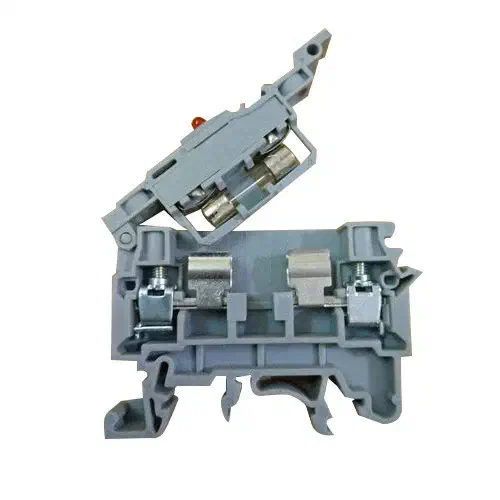
Certain terminals, like the one pictured above, feature an embedded LED indicator that illuminates when the fuse blows. However, unlit blocks are more standard.
You must acquire the correct fuse form-factor (e.g., 5x20 mm glass fuses), rated for the correct voltage and amperage trip threshold.
A critical engineering caveat: the market is flooded with 230 V AC fuses. Can they be safely deployed on DC lines?
Absolutely. When a fuse blows during a fault, an electrical plasma arc forms. In an AC circuit, the sinusoidal wave passes through the zero-crossing, effectively extinguishing its own arc.
In a DC circuit, the arc is vastly more aggressive, and a low-rated AC fuse might fail to break the circuit. However, since our PELV bus is only 24 V DC, standard 230 V AC fuses are perfectly capable of rupturing the arc at this voltage level.
Our PSU delivers a maximum of 3.125 A according to specifications.
The PLC outputs are fused at 2 A, providing a generous power margin for future I/O expansion.
(One might worry about the inrush current of the contactor’s DC coil. However, pure DC coils exhibit practically zero inrush current. Their current draw is strictly governed by the active ohmic resistance of the copper winding. Unlike AC coils – which suffer massive inductive inrush before the magnetic core snaps shut – a DC coil immediately settles at its nominal holding current).
Furthermore, highly advanced modules exist explicitly for segmenting 24 V buses! They are known as “Electronic Circuit Breakers” (ECB) or “Selectivity Modules”.
The keyword is “Electronic”; they utilize high-speed MOSFET logic to sever a faulted channel in microseconds, vastly outperforming melting thermal fuses.
With ECBs, there is no need to physically swap blown fuses. Moreover, the trip threshold is programmable per channel! If a fault occurs, a diagnostic LED illuminates for the specific branch.
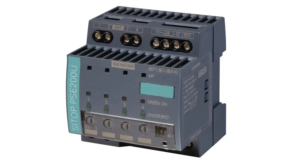
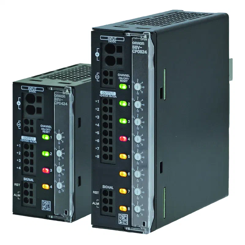
Be advised: these modules require their own baseline operating voltage. A severe undervoltage event can disrupt their internal logic, potentially failing to guarantee channel disconnection during a fault.
Thus, the 24 V Control tier layout (left to right):
- 24 V “+” Distribution block;
- Four fused feed-through terminal blocks – one for each control segment;
- 0 V “-” Distribution block;
- PLC RS-485 expansion module:
Siemens S7 241-1CH32-0XB0; - Siemens S7 1214C PLC, part number
214-1AG40-0XB0. The industry standard, perfectly suited for our objective; - Safety Relay
Omron G9SA; - Contactor
Siemens Sirius 3RT2015-1BB42.
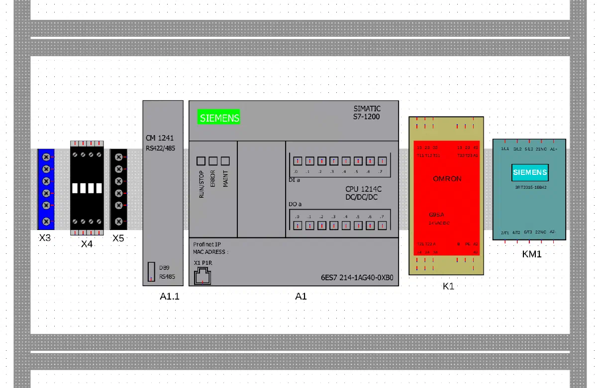
Finally, the operator interaction panel and pendant tier:
- Feed-through terminal blocks for routing the remote pendant;
- DIN-rail socket to simulate the physical load;
- Socket voltage presence indicator light
CHINT ND16-22DS/4; - E-Stop Button
CHINT NP2; - Remote control pendant (Pushbutton station) utilizing
Leudinox LA38switches.
The final spatial layout of our control cabinet:
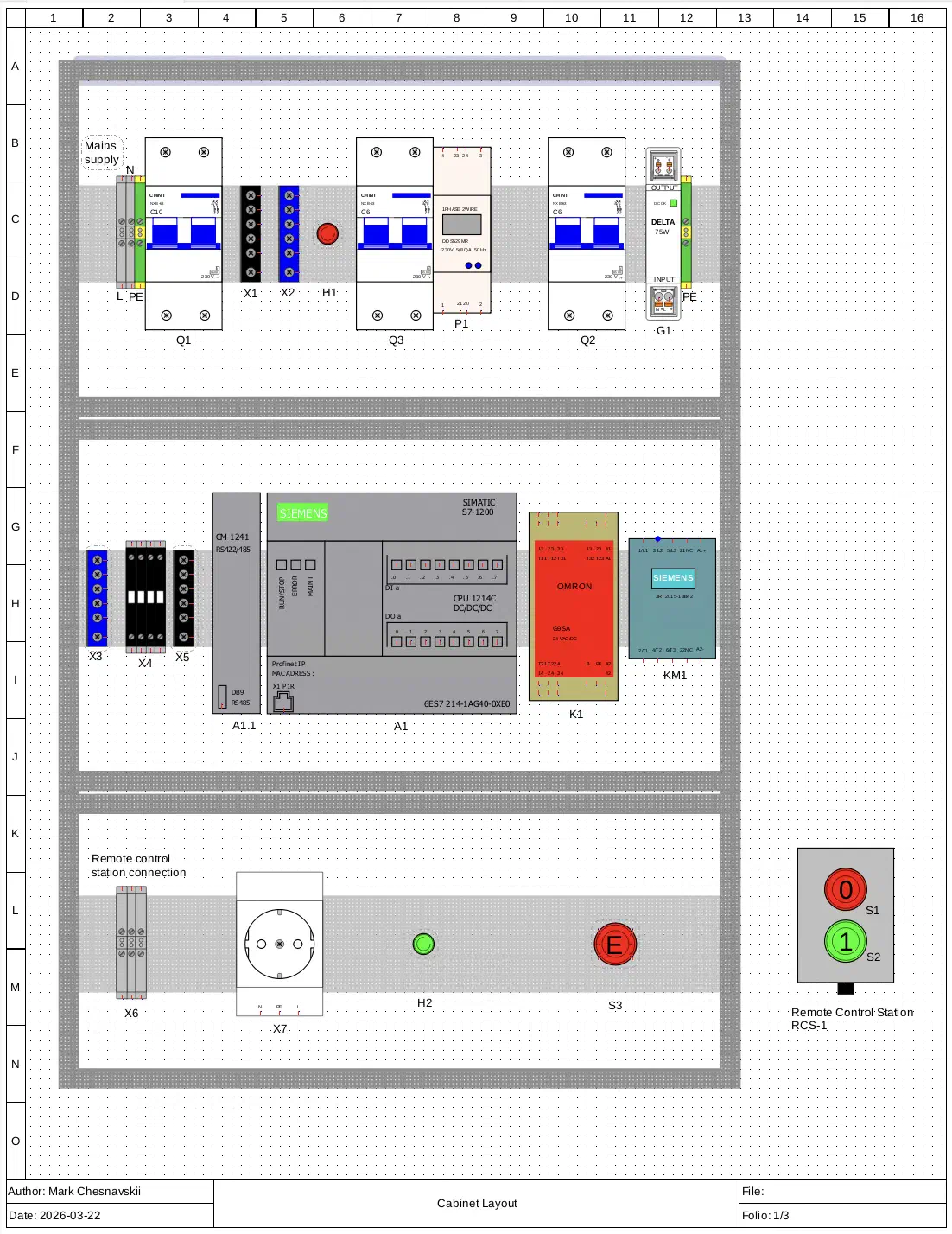
Notice that all cabinet elements are tagged with standard alphanumeric designators. This ensures a 1:1 mapping between the physical layout and the electrical wiring diagram.
According to the IEC 81346 standard:
| Device Category | Letter Code |
|---|---|
| Circuit Breaker | Q |
| Contactor | KM |
| Safety Relay | K or A |
| Control Switches / Pushbuttons | S |
| Visual Indicators (Lamps) | H |
| Power Supply Unit (PSU) | G or U |
| Energy Meter | P |
| PLC (Programmable Logic Controller) | A or K |
| Socket / Plug connector | X |
| Terminal Blocks / Distribution Bars | X |
3.2. Wiring Diagram
The next logical phase is to draft the complete electrical schematic. Attempting to superimpose this onto the layout
diagram is highly impractical, so we return to QElectroTech and create a new Folio → rename it Electrical Schematic.
Review the layout diagram. At the input of the power tier, we have three feed-through terminal blocks labeled “Mains supply”. The main power cord (from a wall socket, in our case) connects here.
In the wiring diagram, we will use a “Single-pole source + PE + N” element. The phase (Line) and Neutral are connected to breaker Q1. By convention, the input (line side) of a circuit breaker is fed from the top terminals. Standard wiring practice dictates Phase on the left, Neutral on the right.
Downstream of the breaker, we install distribution blocks for Phase and Neutral – these will serve as our 220 V bus.
We label each component according to the designators established on the layout diagram. Pay close attention to the circuit breaker symbol – it is a 2-pole device, with each pole featuring both a magnetic release (the square step) and a thermal release (the semicircle arc at the bottom):
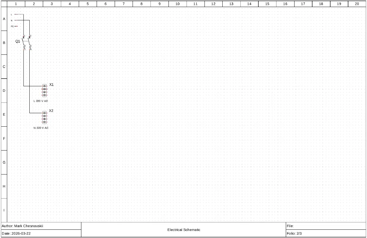
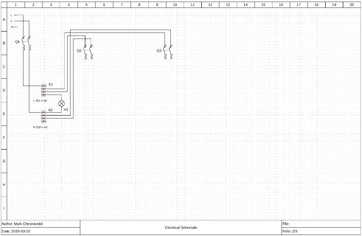
Next, we connect the H1 indicator lamp – it operates directly on 220 V. It is critical to note that the lamp is wired in parallel to the main bus, not as a “pass-through” element. The main power circuit to the load must not pass through the indicator’s contacts.
Then, we wire breakers Q2 and Q3 to the 220 V bus. Input at the top, load (output) at the bottom. Phase left, Neutral right:
Continuing with the power line. Downstream of breaker Q3 is the energy meter, P1.
Different energy meters have different terminal layouts. On our chosen model, SinoTimer DDS529MR, Neutral is at the
top, Phase at the bottom. Input is on the left, output is on the right.
The meter’s output is routed to the main power contacts of contactor KM1 (which we will label shortly) – the element is called “Contact power contactor”.
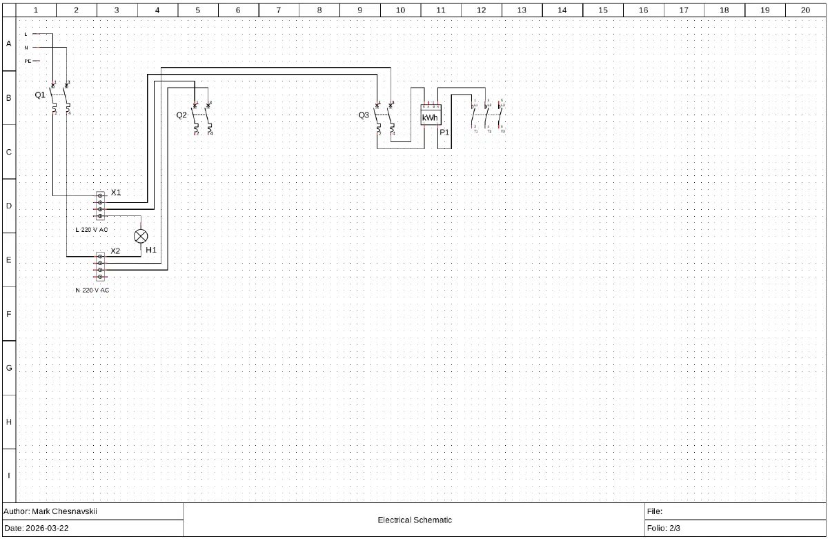
Examine the contactor’s symbol. A contactor has a control coil and power contacts.
Despite being physically co-located within a single housing, they are schematically separated: the power contacts are drawn on the power circuit (as shown above), while the coil is drawn separately on the control circuit (as we will see shortly).
Observe the designation of the power contacts. The horizontal dashed line linking the contacts signifies that all three poles actuate (close/open) simultaneously.
This is a classic three-pole contactor (for a 3-phase load).
Single-Phase vs. Three-Phase Power
Residential Single-Phase Grid
Residential grids utilize single-phase power: one phase and a neutral.
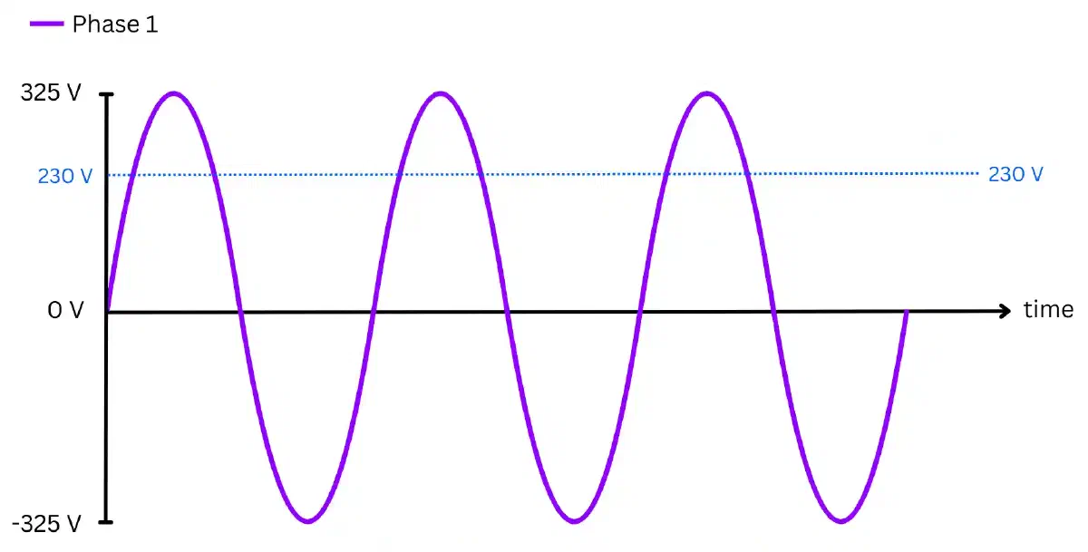
The voltage on the phase wire follows a sinusoidal waveform at 50 Hz – current effectively oscillates back and forth between the source and the load. The neutral wire serves as a reference point and return path.
The RMS (Root Mean Square) voltage is ~220-230 V; the absolute peak voltage of the sine wave is ~325 V.
Industrial Three-Phase Grid
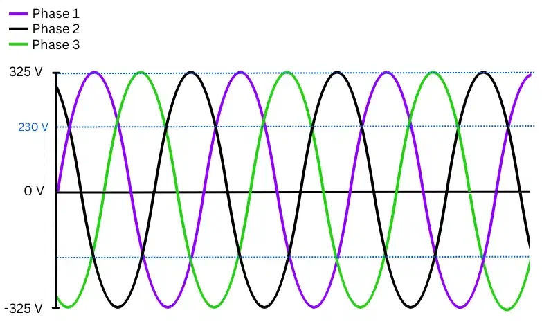
A three-phase grid utilizes three phase lines, each shifted 120° relative to the others. The voltage between any phase and neutral is still ~220 V (RMS), but the voltage between any two phases is ~380 V (RMS).
This is a direct result of the phase shift: at any given moment, one phase might be positive while another is negative, resulting in a larger potential difference between them. This is visually evident on the graph:
This phase shift provides a critical advantage: when the three windings of an electric motor are connected to the three phases, a rotating magnetic field is generated.
The windings sequentially reach their peak, creating a continuous, smooth rotation of the magnetic field without pulsation. This makes three-phase power ideal for electric motors (elevators, pumps, HVAC, etc.).
Single-phase motors are also widely used (e.g., in home appliances; refrigerators connect to single-phase power). They use a phase-shifting start capacitor to create a “pseudo-phase” for startup, but this solution is less efficient and provides inferior starting and running characteristics.
To emulate our load, we are using a DIN-rail socket and a single-phase device. Therefore, we will only utilize two of the contactor’s three power contacts – to break both the phase and neutral lines.
We complete the power line wiring – the contactor’s output is wired to the socket and the indicator lamp, in parallel. Remember that the socket must be grounded (Protective Earth).
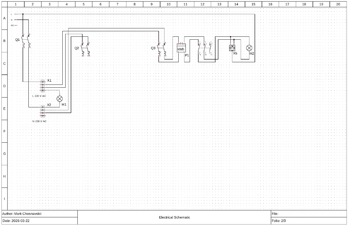
Strict regulatory requirements for the physical position of phase-neutral contacts in a socket are not universal and must be verified for each country. Often, it’s a matter of established best practices.
Example: A bedside lamp may have a single-pole switch that only breaks the phase line. If phase and neutral are reversed in the socket, accidentally touching the threaded part of the bulb socket while changing a bulb will result in a lethal electric shock, even if the switch is in the “OFF” position.
The output of breaker Q2 is connected to the power supply unit G1, which converts 220 V AC to 24 V DC. At the PSU’s output, we install distribution blocks – a 24 V DC bus (X3) and a 0 V DC bus (X5).
To the X3 distribution block, we connect four fused feed-through terminal blocks – one for each dedicated control line:
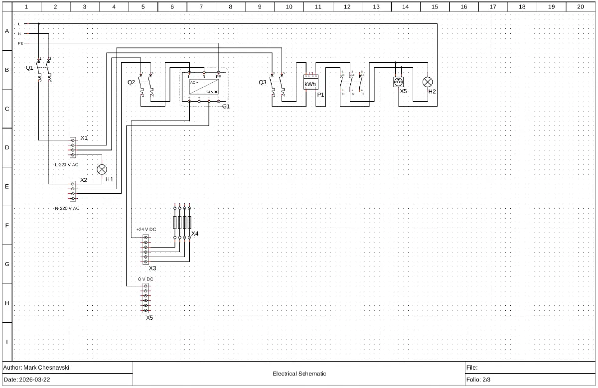
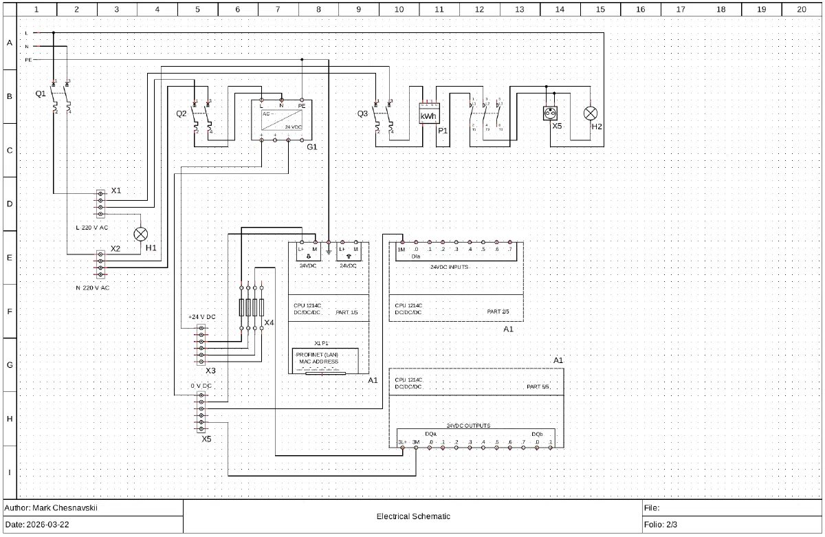
It is time to wire the PLC. For schematic clarity, different functional parts of the PLC are broken down into modules – even though they are part of a single physical device – power input, ground, Ethernet port, digital inputs, analog inputs, and digital outputs.
In QElectroTech, the schematic blocks for the controller are located in Electric → Manufacturers articles → Siemens → PLC and controllers → 6ES7-1200 → CPU1214C 6ES7214-XXXX-0XB0 PARTX.
It is absolutely critical to ground the PLC (A1)! Failure to do so can lead to a situation where the controller randomly throws peripheral initialization faults on startup. Without a solid ground connection, the PLC’s internal EMC filters operate erratically, and all induced noise is shunted directly into the CPU and the RS-485 expansion board.
What are EMC filters?
EMC stands for Electromagnetic Compatibility.
EMC filters are circuits designed to suppress electrical noise. They perform two functions:
- Prevent external noise from entering the device (from the grid/cables);
- Prevent internal noise from escaping the device (into the grid).
Specifically, they:
- Attenuate high-frequency noise;
- Shunt this noise to ground (PE);
- Smooth out voltage spikes.
Therefore, a missing ground connection can lead to PLC startup errors. To prove this at a hardware level, we would need an oscilloscope and a high-frequency current clamp.
In a future article, we will clamp the ground wire and witness this noise pulse with our own eyes during startup.
Next:
- Connect 24 V DC to terminal “L+”, and 0 V DC to terminal M – this powers the PLC itself;
- Connect 0 V DC to terminal 1M – the common negative for the digital inputs;
- Connect 24 V DC to terminal “3L+”, and 0 V DC to terminal 3M – this powers the digital outputs;
- Ground the PLC (!).
The PLC wiring appears as follows:
Now we wire the safety relay, K1. As previously discussed, the safety relay has its own dedicated power feed from our segmented 24 V DC bus:
- Relay terminal A1 connects to the 1 A fused terminal block;
- Terminal A2 connects to the 0 V DC bus;
- The relay is grounded via the PE terminal.
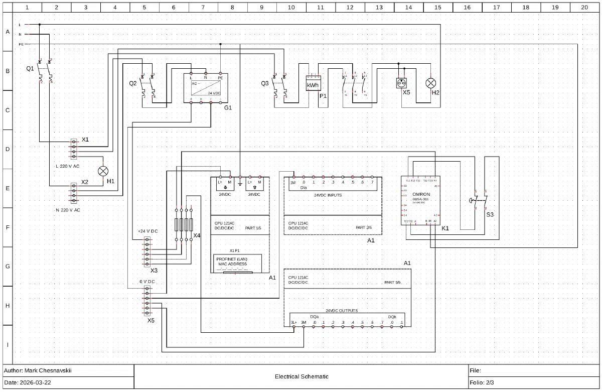
Next, we wire the E-STOP button (S3) with its two NC (Normally Closed) contacts to the relay.
First emergency stop signal channel:
- Relay terminal T11 is wired to the “input” of the first button contact: 1;
- Relay terminal T12 is wired to the “output” of the first button contact: 2.
Second emergency stop signal channel:
- Relay terminal T21 is wired to the “input” of the second button contact: 1;
- Relay terminal T22 is wired to the “output” of the second button contact: 2.
Thus, the E-Stop button is placed in-line, breaking the T11-12 and T21-T22 safety relay circuits:
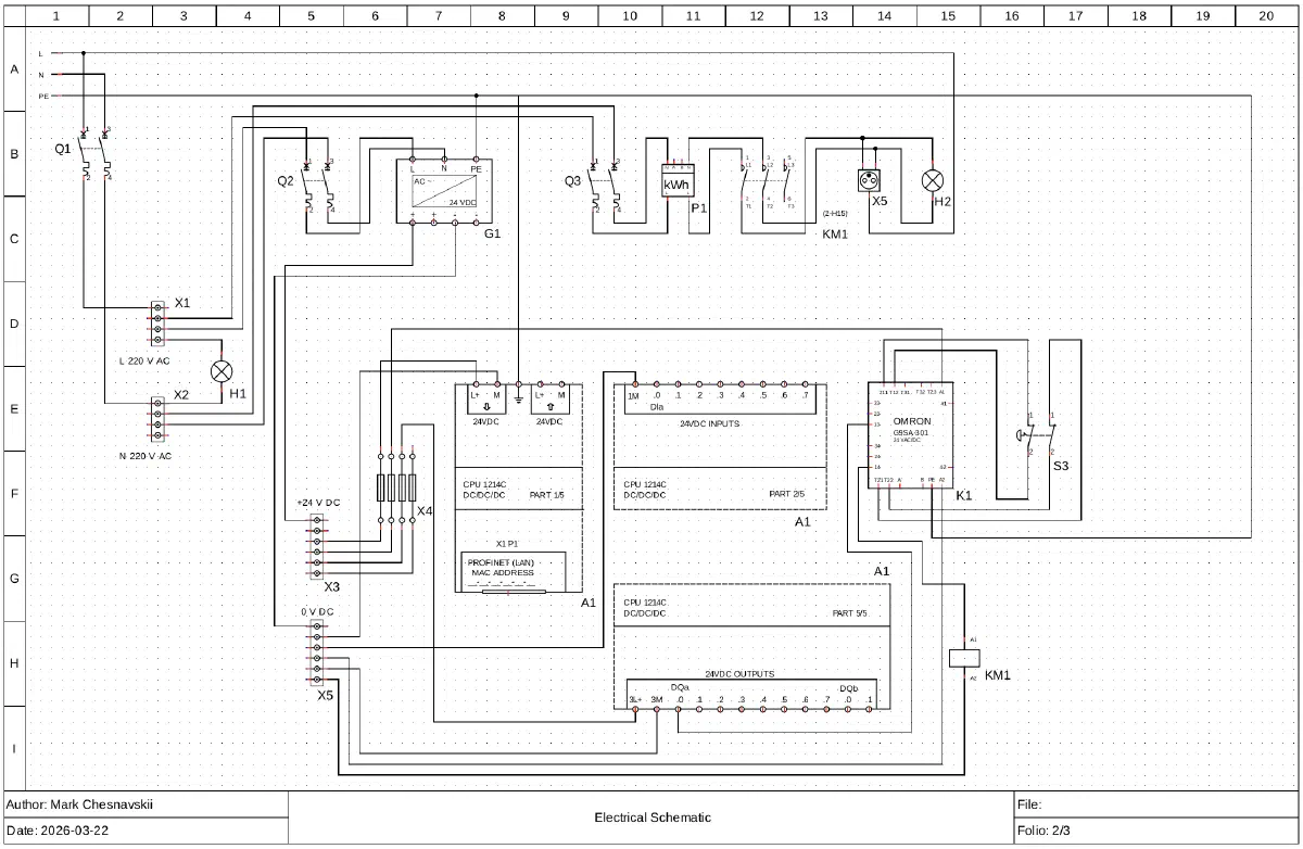
We add the contactor’s coil to the schematic. The PLC controls this coil, and the safety relay makes or breaks the circuit as needed:
- Connect the PLC’s digital output 0 (Q0.0) to terminal 13 on the safety relay;
- Terminal 14 of the relay goes to terminal A1 of the contactor coil (the “+”);
- Terminal A2 of the coil connects to the common 0 V DC bus.
Linking the Coil and Contacts
Since the contactor’s power contacts and its control coil appear in different locations on the schematic but are physically part of the same device, we must link them in the software:
- Double-click the coil → “Information” tab → Label → name it
KM1; - Double-click the power contacts → in the new window, find KM1 → Link the item → Apply.
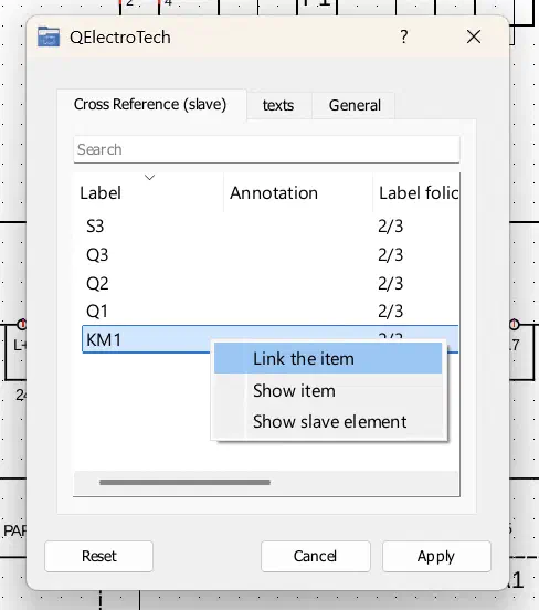
QElectroTech will automatically place a “KM1” label on the power contacts. Additionally, next to the power contacts, a
cross-reference will appear indicating the schematic coordinates of the coil, e.g., 2-H15, which means: Folio 2 →
column 2 → row “A”.
When you hover over one part of the contactor, the other part will automatically be highlighted, significantly simplifying schematic navigation.
Pro Tip: If you try to move an element’s label in QElectroTech, the entire element moves. To move just the label, you must first hold down the Shift key.
The PLC controls the coil, with the safety relay acting as a hardwired interlock in the control circuit:
Now for a critical step – wiring the flyback diode. Early in the article, in the section on contactors, we established that de-energizing a contactor’s coil generates a back-EMF spike on the order of 100-1000 V.
The magnitude of the EMF spike is proportional to how sharply the control signal is cut. A PLC’s solid-state transistor output switches extremely fast, exacerbating the spike. In subsequent articles, we will measure this spike with an oscilloscope to analyze its waveform, amplitude, and duration.
Such a spike can easily cause dielectric breakdown and destroy the transistor.
The simplest way to protect the control line when de-energizing a DC coil is to connect a 1n5408 diode in parallel
with the coil, in reverse bias: the diode’s cathode to the coil’s anode, and the diode’s anode to the coil’s cathode.
As a result, the back-EMF spike is shunted back into the coil, where the energy circulates until it is dissipated as heat by the coil’s own resistance: $$ P = I^2R $$
This solution perfectly protects sensitive electronics, but it has a trade-off. Specifically, the coil de-energizes more slowly because the collapsing magnetic field’s energy is fed back into it. The coil continues to hold the contactor’s armature closed for a fraction of a second longer, reducing the contactor’s “aggressiveness” – the circuit breaks more slowly.
Back-EMF Suppression Methods
Diode (DC Flyback)
- Completely suppresses the back-EMF spike;
- Drawback: The coil’s current decays slowly → longer de-energization time.
RC Snubber (Resistor + Capacitor in series, parallel to the coil)
- Current decays faster → faster switching time;
- Drawback: Does not fully suppress the spike; small voltage peaks remain.
Varistor
- Absorbs peaks but is poorly suited for DC circuits;
- Under normal conditions, a varistor has very high resistance and passes almost no current;
- When voltage exceeds a certain threshold, its resistance plummets, “clamping” the voltage spike by absorbing the energy;
- Primarily used for protection against short, high-energy transients, especially in AC grids;
- Under constant DC or prolonged overvoltage, a varistor will overheat and degrade over time.
RCD Network (Resistor + Capacitor + Diode)
- A balanced approach: almost completely suppresses EMF while allowing the coil to de-energize faster than with a diode alone.
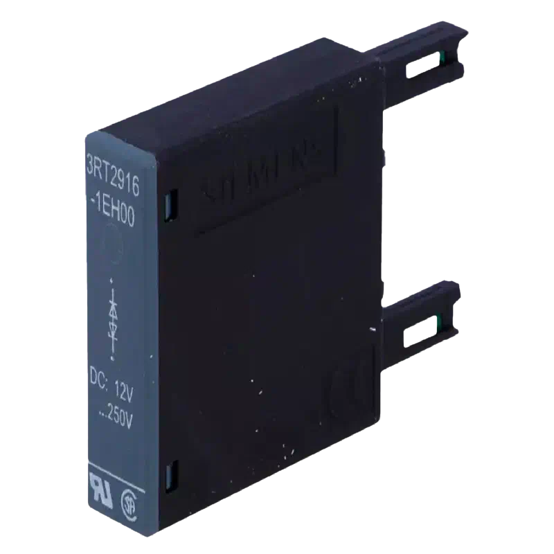
Contactor manufacturers produce ready-made modules that snap directly onto the face of the contactor, for example, the
Siemens 3RT2916-1EH00 – a diode-based variant:
We connect the DC flyback diode D1 in parallel with the KM1 coil, in reverse bias:
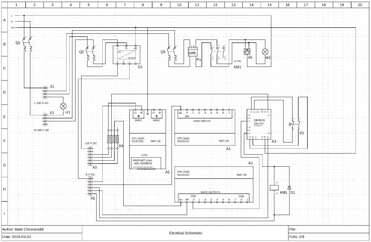
It gets more interesting. The K1 safety relay defaults to a tripped state and will not permit the control signal to pass.
Furthermore, if the E-STOP button is pressed, the relay also enters a tripped state and breaks the control circuit until it is subsequently reset.
We must explicitly close (and then open) the T31-T32 terminals; for the relay, this signals: “all clear, the system is ready for startup”.
This reset signal can come from a dedicated “reset” button on the operator panel, or from an EDM loop – External Device Monitoring / Feedback Loop.
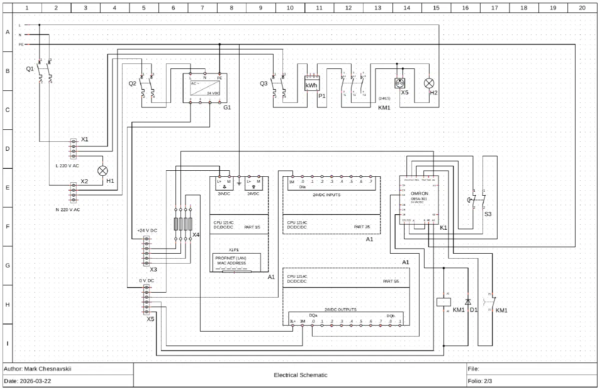
Our contactor has auxiliary NC contacts, 21NC and 22NC, which open when the main power contacts close. That is: contactor energized → 21NC-22NC circuit is open. Contactor de-energized → 21NC-22NC circuit is closed.
EDM and Safety Relay Reset
External Device Monitoring (EDM) is an operational mode where the relay sends a signal out from T31 and expects it to pass through all the NC auxiliary contacts of the system’s contactors and return to T32. If any contactor has “welded” its contacts shut, the signal will not return, and the relay will enter a fault state.
By routing the relay’s reset circuit T31-T32 through the contactor’s 21NC-22NC contacts, the relay gains knowledge of the contactor’s physical state. If the contacts are stuck, startup permission will be denied.
There is a nuance here: by default, the relay reacts to a falling edge on the T31-T32 circuit:
- The relay is in a tripped state;
- We close the T31-T32 circuit ← nothing happens at this stage;
- We open the T31-T32 circuit ← the relay resets at this moment.
Upon system power-up, the contactor’s main contacts are (normally) open, meaning its auxiliary NC contacts are closed. If we connect 21NC-22NC to T31-T32, the reset condition (opening the circuit) will never be met, and the relay will never exit its tripped state.
The key is that the relay has two reset modes:
- Manual (triggered by the falling edge from a button);
- Automatic (for EDM).
Switching between modes is done by opening or closing terminals A and B on the safety relay:
- If terminals A and B are open, the relay operates in manual reset mode;
- If terminals A and B are connected with a jumper, the relay operates in feedback loop mode and reacts to a rising edge on the T3-T32 circuit.
The auxiliary 21NC and 22NC contacts of the contactor can be represented by an “Electromagnetic relay NC” element in QElectroTech. It is critical to label this element as belonging to contactor KM1.
We connect relay terminal T31 to 21NC on the contactor, and 22NC on the contactor to T32 on the relay. Then, we directly jumper terminals A and B on the relay.
This results in the following schematic:
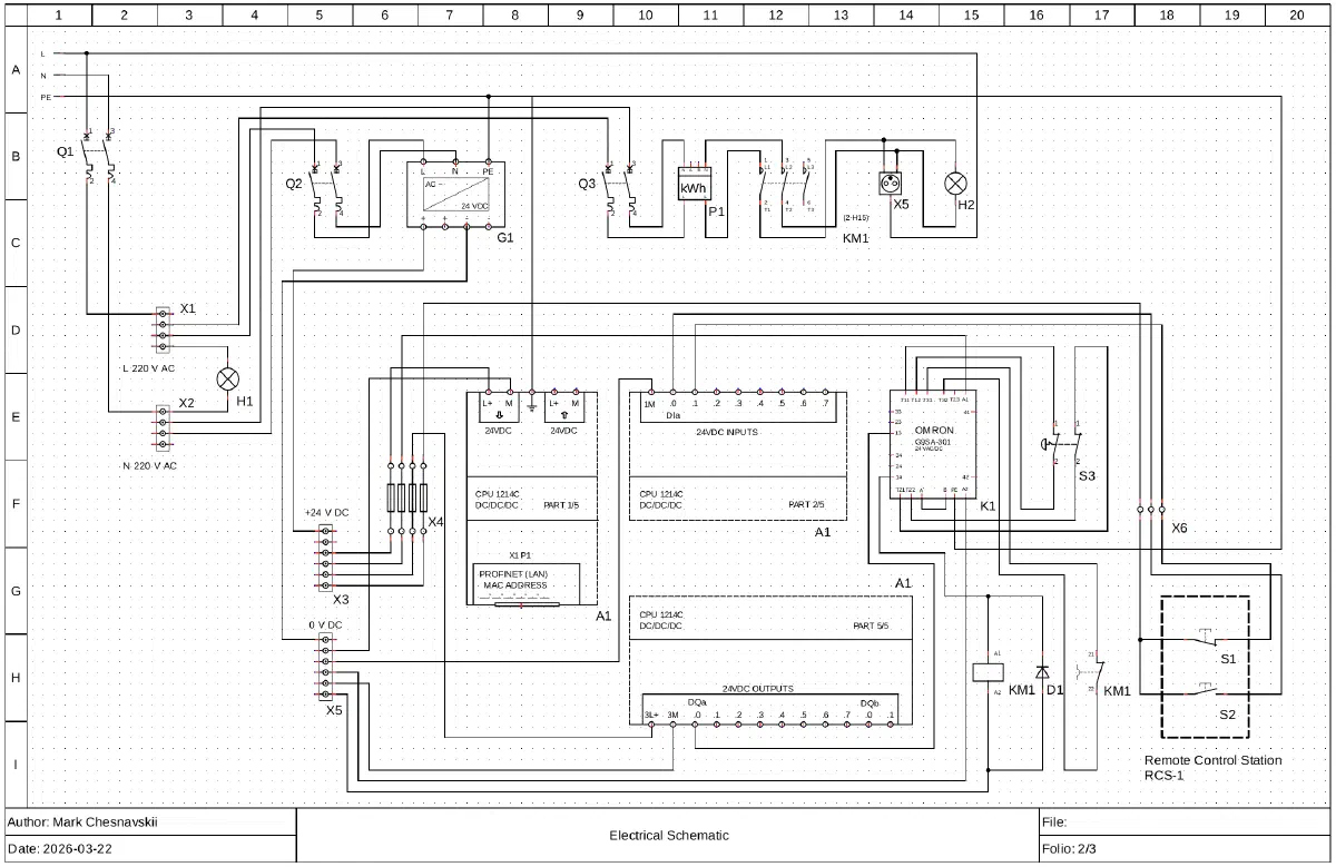
We connect the RCS-1 pushbutton station with buttons S1 (“STOP”) and S2 (“START”):
- Feed-through terminal blocks X6 – these are for the remote pendant’s cable;
- To one of the terminals, we connect 24 V DC from its dedicated fuse;
- The other two terminals – the “return” control signals from the buttons – are connected to the PLC’s digital inputs 0 and 1.
The schematic with the RCS-1 pushbutton station connected:
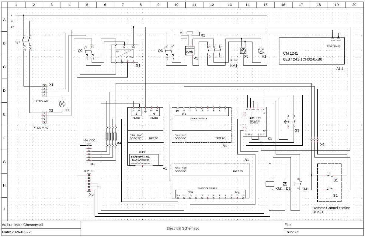
All that remains is to connect the energy meter P1 to the PLC’s RS-485 expansion board (A1.1)!
The meter has terminals A and B. They must be connected to the T/R+ and T/R- pins on the RS-485 board.
Unfortunately, the A/B labeling standard is frequently violated, so empirical testing is often required:
- Connect
A→T/R+andB→T/R-. If it works, you are done. - If not, reverse the polarity:
A→T/R-andB→T/R+.
The RS-485 bus uses differential signaling, meaning data is transmitted as the voltage difference between wires A and B. When a signal reaches the end of the line, it reflects back, creating distortion and communication errors.
This problem is solved by installing a terminating resistor at the end of the bus. A 120 Ω resistor on the last device “absorbs” these reflections and stabilizes the transmission. We connect resistor R1 in parallel across the A and B terminals of the energy meter.
The final wiring diagram for the control cabinet:
4. Bill of Materials and Procurement
QElectroTech features a built-in BOM generation tool. To use it:
- Open the wiring diagram;
- Double-click each component;
- Populate the label, manufacturer, and article number fields;
- Navigate to Project → Export to CSV.
The Bill of Materials (BOM) for our cyber-physical testbed is as follows:
| Designator | Manufacturer | Part Number | Description | Qty |
|---|---|---|---|---|
| A1 | Siemens | 6ES7 241-1AG40-0XB0 | PLC CPU 1214C | 1 |
| A1.1 | Siemens | 6ES7 241-1CH32-0XB0 | RS-485 Communication Module | 1 |
| D1 | Nubbeo | 1n5408 | Diode 1N5408 | 1 |
| G1 | Delta | DRL-24V75W1AZ | DC Power Supply Unit | 1 |
| H1 | CHINT | ND16-22DS/4 | Indicator, Red | 1 |
| H2 | CHINT | ND16-22DS/4 | Indicator, Green | 1 |
| K1 | Omron | G9SA-301 | Safety Relay | 1 |
| KM1 | Siemens | 1P3RT2015-1BB42 | 3-Pole Contactor | 1 |
| P1 | Sinotimer | DDS529MR | RS-485 Energy Meter | 1 |
| Q1 | CHINT | NXB-63 C10 | MCB C10 | 1 |
| Q2..3 | CHINT | NXB-63 C6 | MCB C6 | 2 |
| R1 | Nubbeo | R025-120R | Resistor 120 Ω | 1 |
| S1 | Leudinox | LA38 | Pushbutton, Red, NC | 1 |
| S2 | Leudinox | LA38 | Pushbutton, Green, NO | 1 |
| S3 | CHINT | NP2 | E-Stop Button | 1 |
| X1..3, X5 | Brinna | RU-09/7 | Distribution Block | 4 |
| X4 | Zoloda | BKNP-520 | Fused Terminal Block | 4 |
| X6 | Zoloda | BPN-04-G | Feed-through Terminal Block | 3 |
| X7 | Kalop | KL40245, KL40580 | Socket + DIN Adapter | 1 |
| X8 | WKDO | JUK2 | End Stopper | 10 |
Additional components for the pushbutton station:
| Designator | Manufacturer | Part Number | Description | Qty |
|---|---|---|---|---|
| TB1 | Conextube | HP03 | Cable Gland | 1 |
| TB2 | Sanderson | HJ9-2 | Pushbutton Station | 1 |
Fuses:
| Designator | Part Number | Description | Qty |
|---|---|---|---|
| F1 | F1AL 250 V 5x20 | Fuse 1 A | 3 |
| F2 | F2AL 250 V 5x20 | Fuse 2 A | 1 |
Cabling and Wire Ducts:
| Designator | Cross-section | Color | Type / Purpose | Length |
|---|---|---|---|---|
| C1 | 1.5 mm² | Blue | Flexible multi-strand cable | 12 m |
| C2 | 1.5 mm² | Brown | Flexible multi-strand cable | 12 m |
| C3 | 1.5 mm² | Green | Flexible multi-strand cable | 12 m |
| C4 | 1 mm² | Black | Flexible multi-strand cable | 12 m |
| C5 | 1 mm² | Red | Flexible multi-strand cable | 12 m |
| C6 | 1.5 mm² x3 | - | Flexible industrial cable, 3-core | 3 m |
| C7 | 1 mm² x4 | - | Flexible industrial cable, 4-core | 3 m |
| C8 | - | - | Shielded RS-485 cable, w/ DB-9 | 3 m |
| C9 | 25×25 mm | - | Slotted Wire Duct | 6 m |
Mounting hardware:
| Designator | Mfg. / Type | Description | Size / Qty |
|---|---|---|---|
| XP1 | Richi | Heavy-duty plug w/ cable gland, 10 A | 1 pc |
| C10 | - | DIN-rail, 0.5 m | 3 pcs |
| C11 | - | MDF backplate | 800×560 mm |
| C12 | T1 | Self-tapping screw, washer head | 40 pcs |
Additionally, we will require tools and consumables not listed in the BOM:
- Multimeter;
- Phase indicator screwdriver (voltage tester);
- Precision screwdriver 3.0x50 mm;
- Insulated screwdriver 1000 V PH1X80;
- Utility knife;
- Wire cutters;
- Tape measure;
- Crimping tool with a set of wire ferrules.
Next, we procure all items:
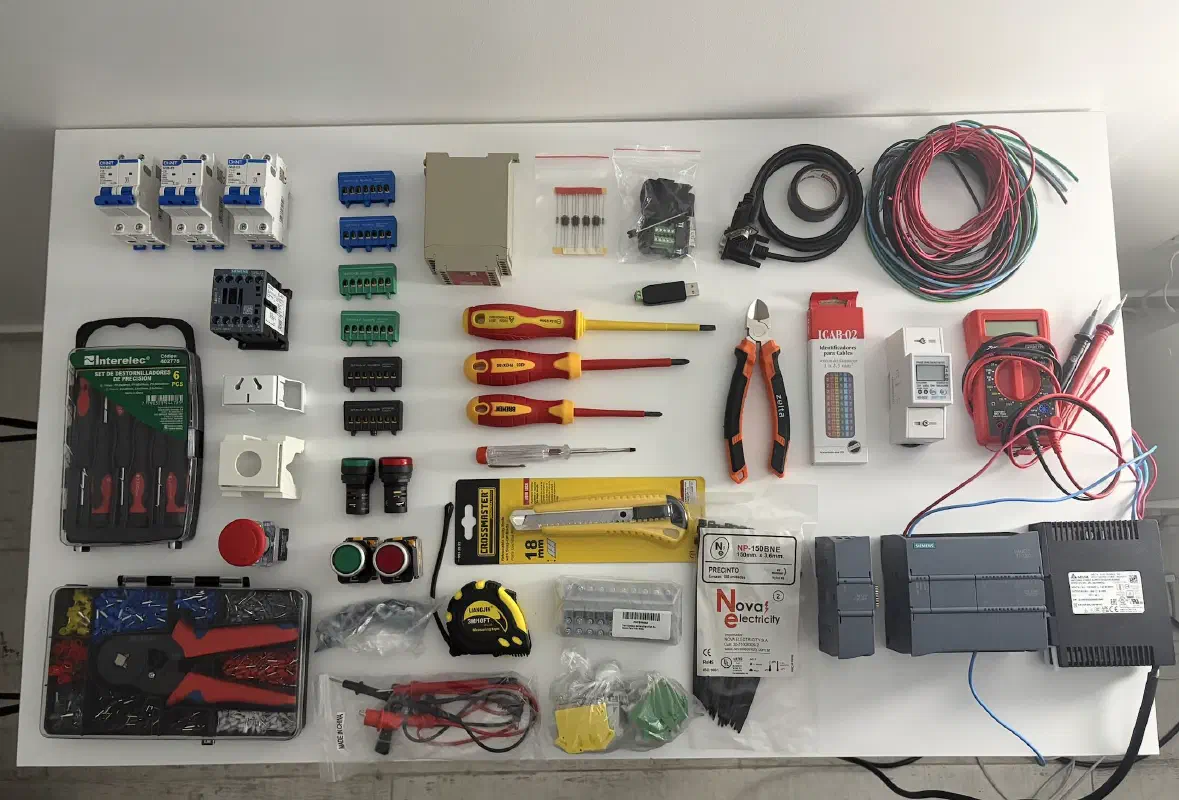
5. Control Cabinet Assembly
Disclaimer: The physical assembly of this control cabinet was performed using C10, C6, and C2 circuit breakers that were available at the time of writing. For a more robust and fault-tolerant system, the C2 breaker should be replaced with a C6, as specified in the schematic.
First, we need an MDF backplate. While an industrial enclosure could be used, our research-oriented work demands easy access and modification, making an open MDF panel a more practical choice:

Mount the DIN-rails and wire ducts:
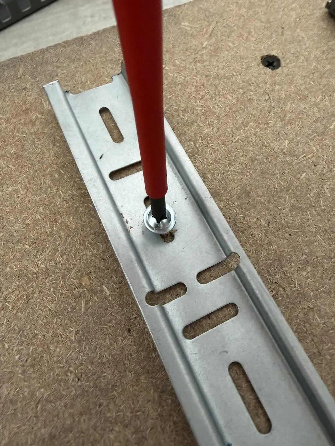
Locate the “Safety instructions → Vertical mounting” section in the Delta PSU datasheet: https://psu.deltaww.com/en/products/download/Datasheet/DRL-24V75W1AZ.
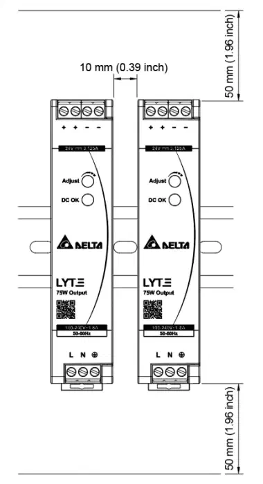
The manufacturer mandates a 50 mm vertical clearance. This is to allow for passive convection cooling: cool air enters from the bottom, passes over the heatsinks, and exits from the top.
We maintain a 50 mm gap between the rail and the wire duct:

Disassemble the power plug:
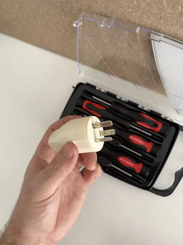
At this juncture, it is critical to state that all stranded copper wires must be terminated with wire ferrules before being clamped into terminals.
If a bare stranded wire is clamped directly, the copper strands will splay and deform over time due to mechanical pressure. This leads to a degraded electrical connection, increased resistance, localized heating, and a significant risk of fire or short circuit.
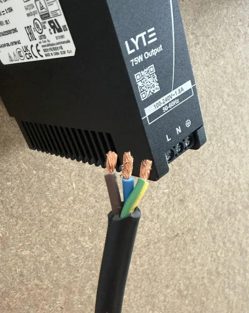
At the time of the initial PLC connection, the wire ferrules had not yet been delivered, so bare wires were used temporarily.
The photo below shows the state of the copper strands after just 7 days: they have splayed apart and deformed.
❌ For any permanent installation, this is absolutely unacceptable.
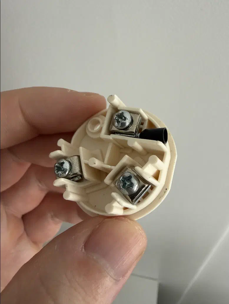
Returning to the plug assembly. What if an insulated wire ferrule does not fit into the plug’s terminal?
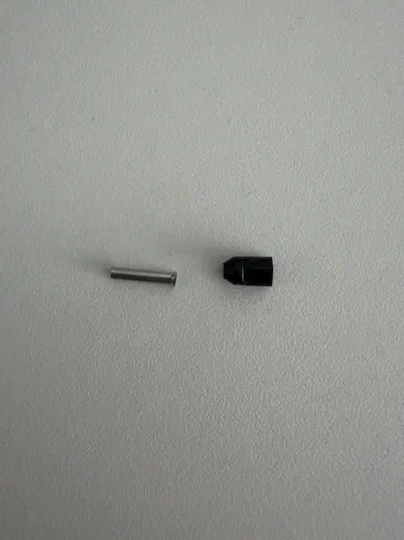
Convert it to an uninsulated ferrule. Take an insulated ferrule and strip off the plastic collar using pliers/cutters:
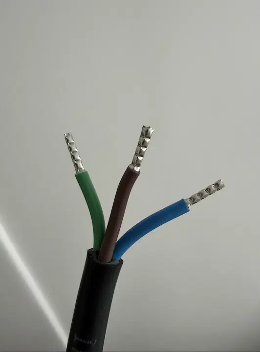
Strip the wire, and (importantly!) without twisting the copper strands, insert them into the ferrule and crimp it with the tool. No bare wire should be exposed.
If the crimped wire still does not fit, the ferrule itself can be trimmed. At this stage, it is crucial to adhere to the local standards for phase and neutral placement in the socket. In some countries, phase is conventionally on the right; in others, on the left.
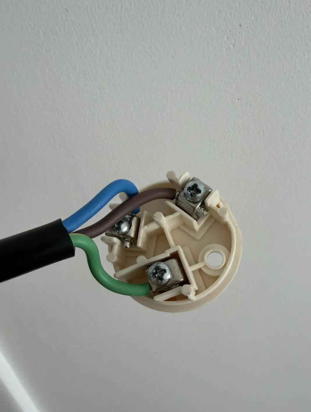
Assemble the plug, securely tightening the cable gland to prevent the wire from being pulled out of the terminals:
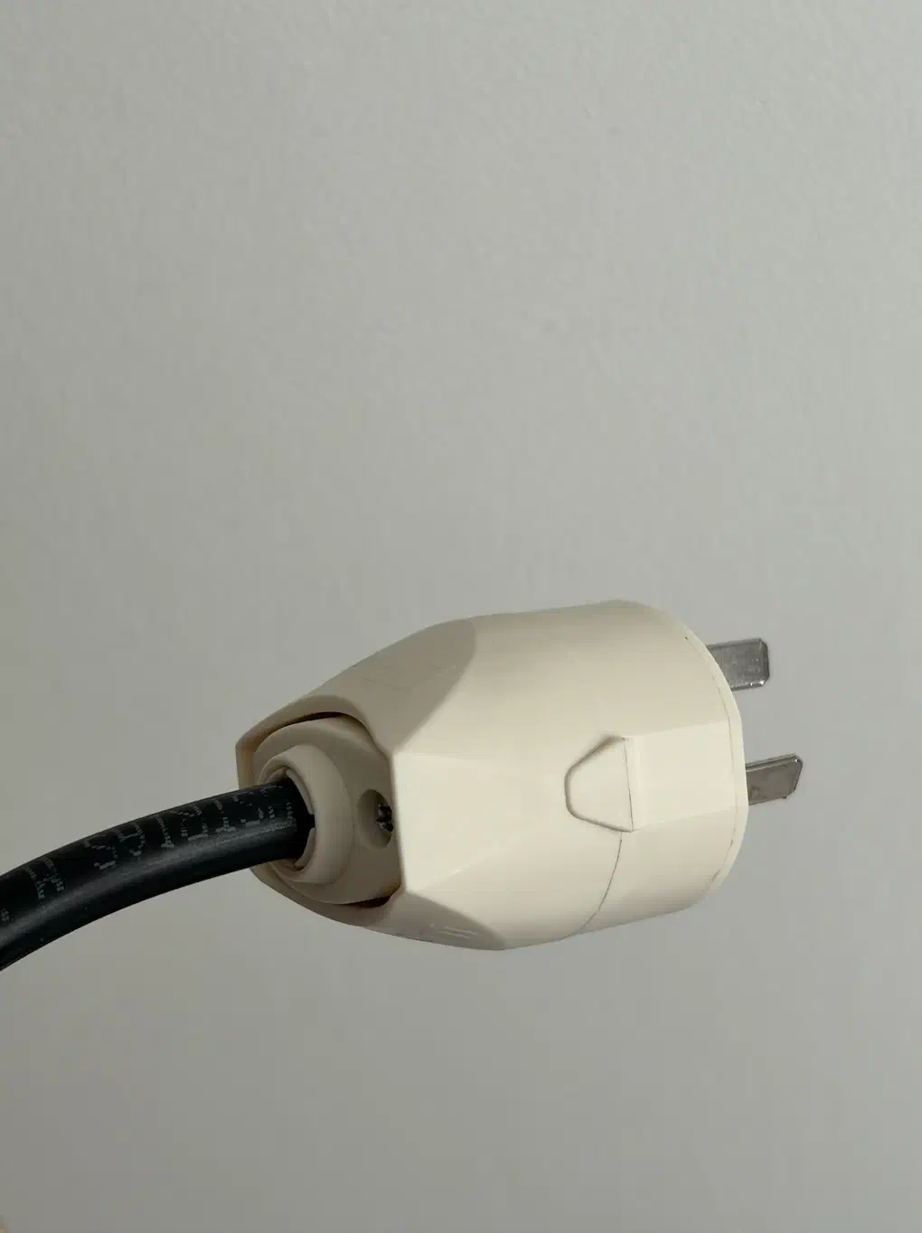
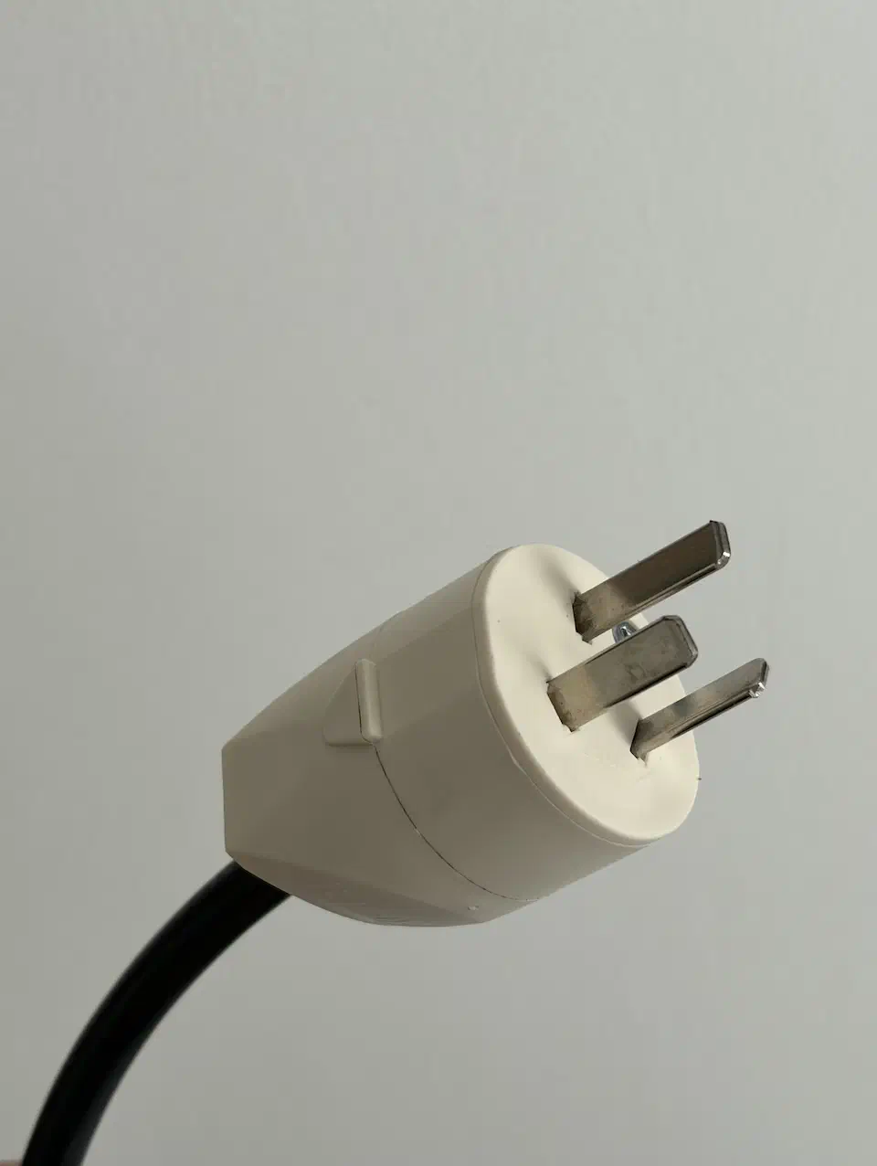
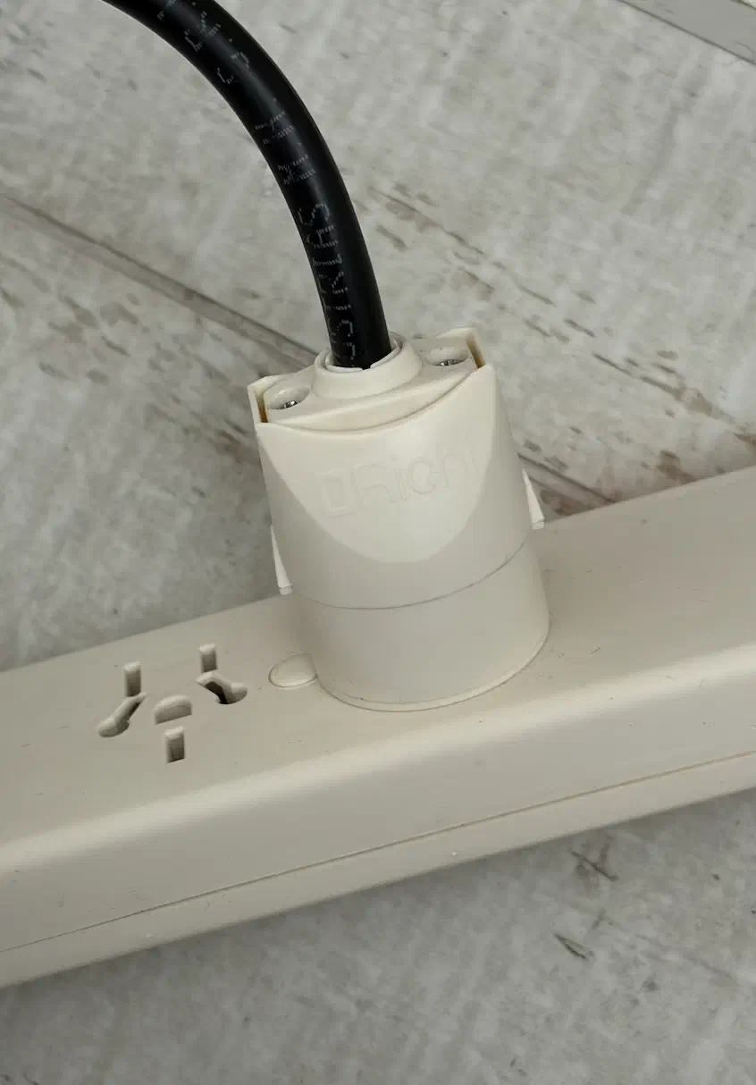
The presence of a PE (Protective Earth) contact in a socket does not guarantee it is actually grounded at the building level! We require a verified ground connection for multiple reasons, both for personnel safety and for system stability.
Recall that the PLC has an EMC filter that shunts electrical noise to ground. The safety relay also requires a ground connection for proper operation.
How to verify if a socket is properly grounded?
️️⚠️️ Before proceeding, you must ensure you are in a focused and competent state of mind. Contact with 220 V AC can induce cardiac arrest.
The principle is to measure the potential difference between phase and neutral, and then between phase and ground. If the ground is connected, the readings should be identical.
If the ground is open-circuit, the voltmeter will read 0 V, as there is no path for the current to flow. A voltmeter has extremely high internal resistance, but its operation relies on a minuscule amount of current passing through it.
- Take safety precautions – eliminate bodily contact with floors and walls.
- Set the multimeter to AC voltage measurement mode, with a limit of at least 750 V.
- Under no circumstances should the multimeter be switched to ammeter mode! This will create a dead short circuit, with risk of electric shock or arc flash. Unlike a voltmeter (connected in parallel), an ammeter is connected in series.
- Measure the potential difference between phase and neutral.
- Measure the potential difference between phase and ground.
Conducting the measurements:
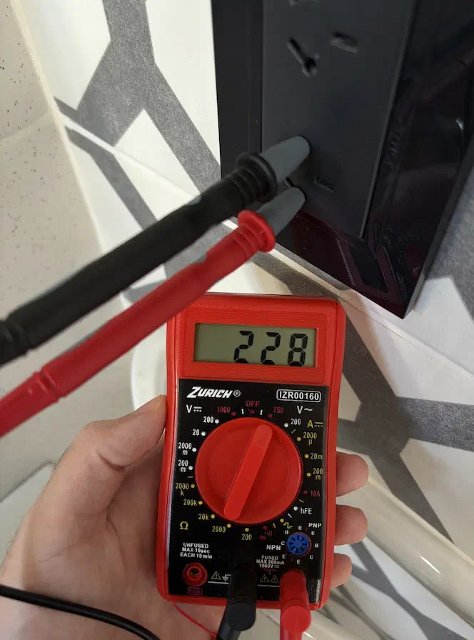
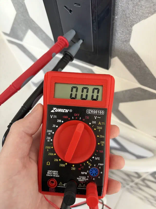
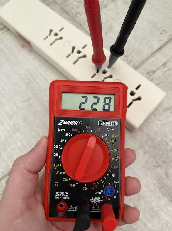
Measurement results:
- First photo
- Grid voltage is 228 V (remember this is the RMS value; an oscilloscope is needed to see the sine wave peaks).
- Second photo
- Potential difference between phase and ground… 0 V! This means this socket is not grounded.
- Third photo
- We measure a different socket and see 228 V; this socket is properly grounded.
It is also necessary to identify which terminal is the phase in the specific socket we will use.
This can be done with a phase indicator screwdriver – it illuminates upon contact with a live phase.
⚠️️ Before drawing any conclusions from a tool’s reading, you must first verify the tool’s functionality. If the tool indicates no phase, it does not mean phase is truly absent. You must perform a control check on a known live circuit to confirm the tool is working correctly.
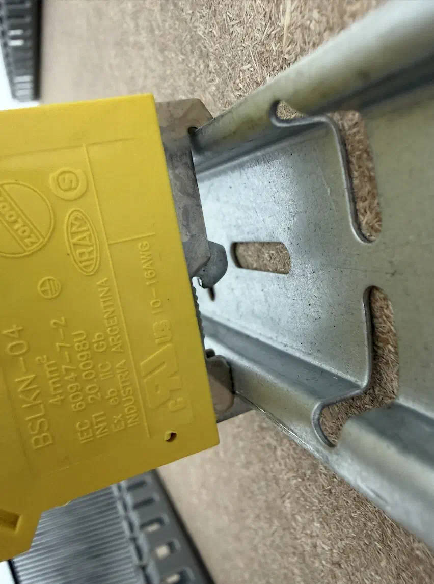
Next, we install an end stopper and the feed-through terminal blocks. Pay special attention to the ground terminal block.
The center of the terminal has a tab that operates the locking mechanism. Lifting it retracts a metal foot, allowing the terminal to be mounted on the DIN-rail.
When installed, the metal foot bites into the surface of the rail, scraping away any oxide layer and ensuring a solid electrical connection.
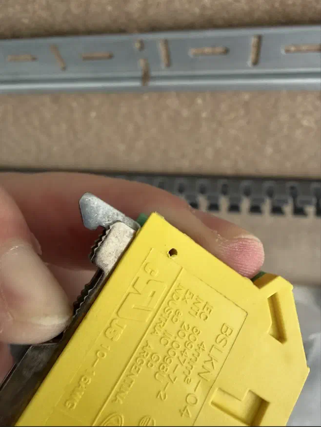

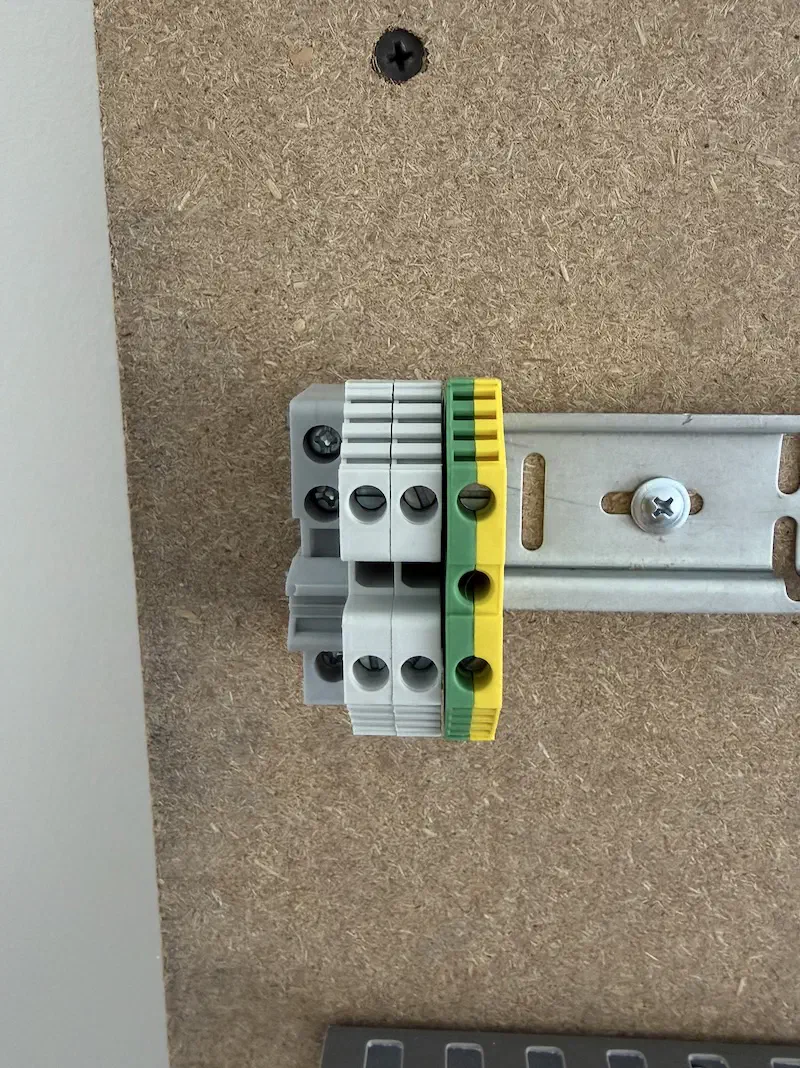
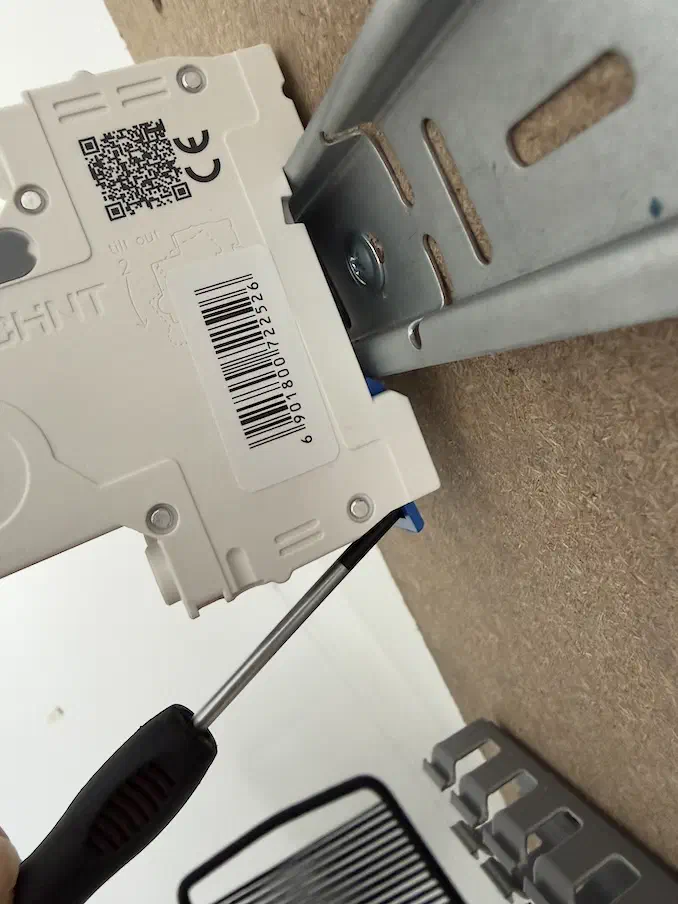
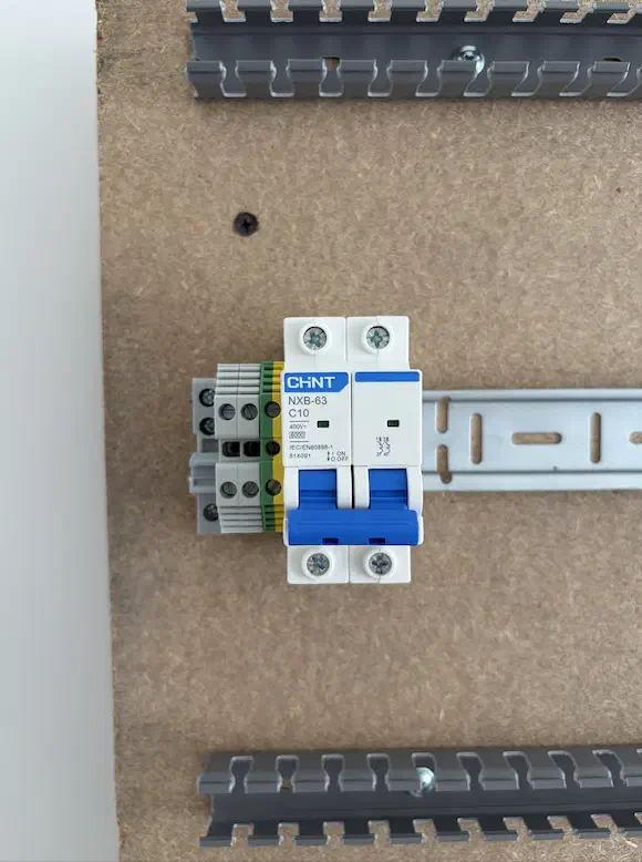
To install the C10 circuit breaker (Q1) on the DIN-rail, hook its top edge over the top of the rail, then pull down the spring-loaded latch, seat the bottom edge on the rail, and release the latch to lock it in place:
Install the indicator lamp into its DIN-rail adapter:
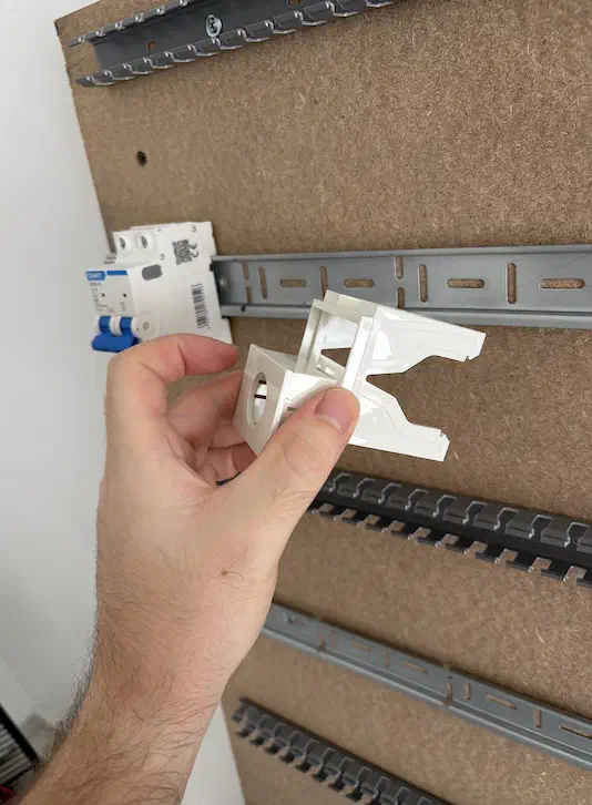
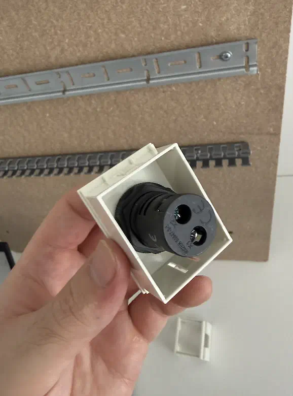
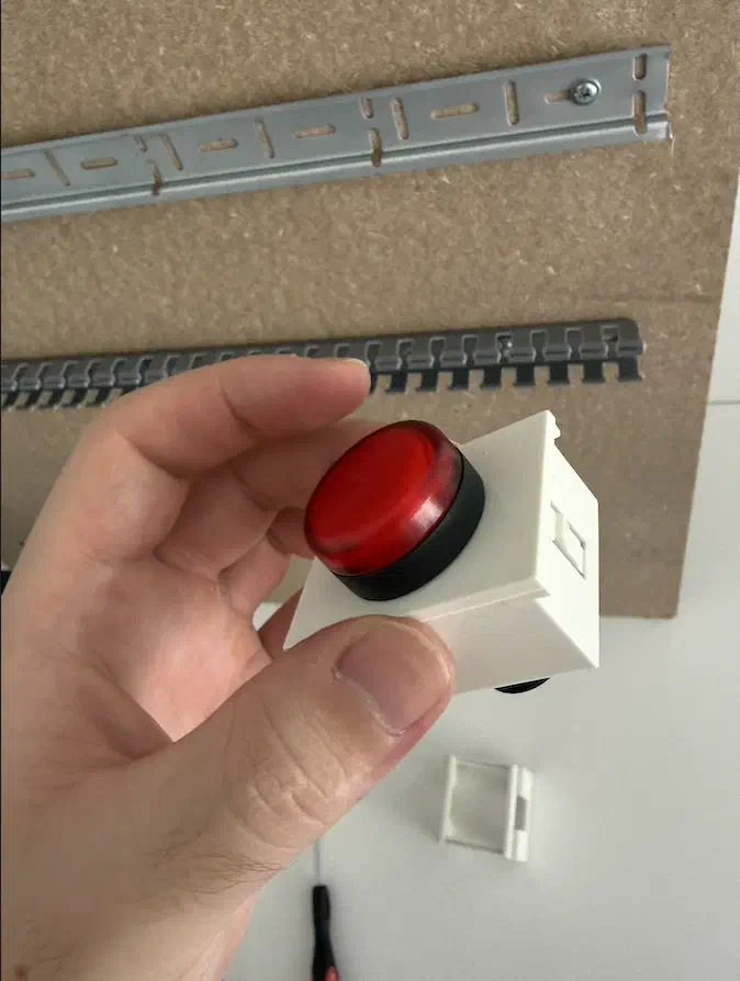
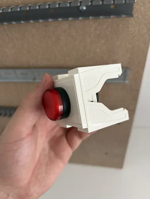
Install the E-STOP button (also known as a “mushroom head”) into its DIN-rail adapter:
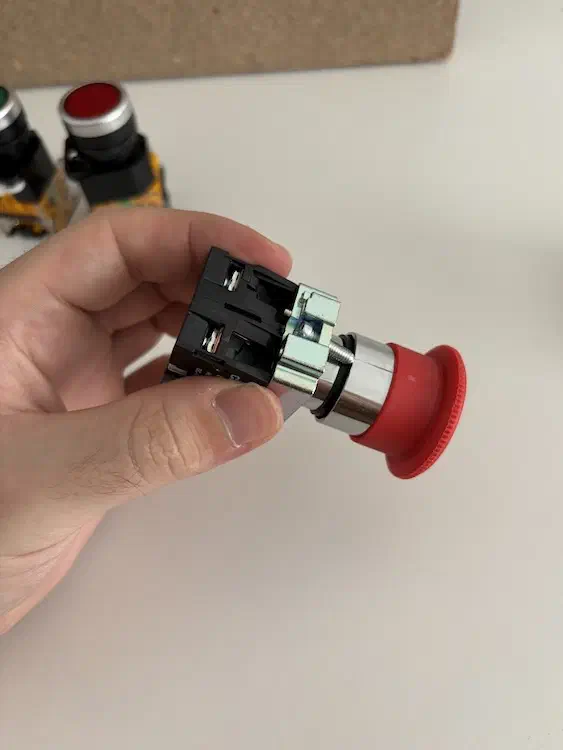
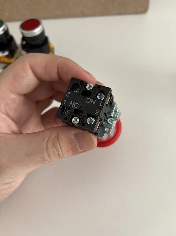
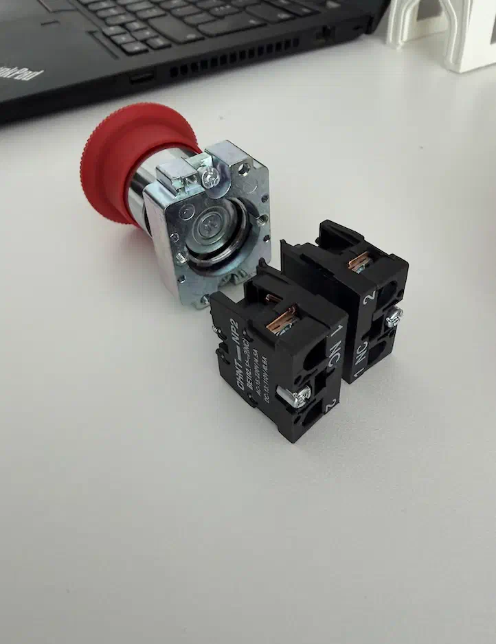
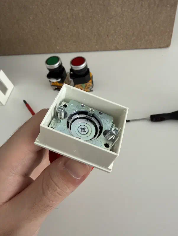
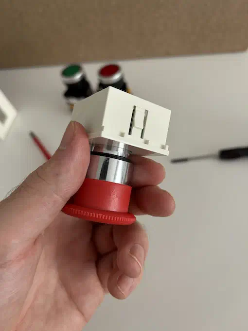
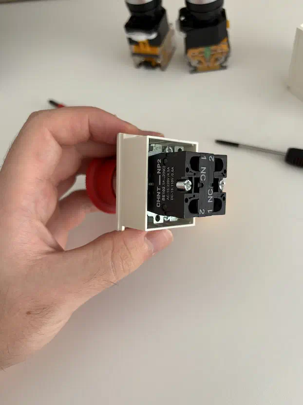
Begin wiring the components according to the schematic. Use 1.5 mm² wire for the power lines and 1.0 mm² for the control lines. Crimp all stranded wires with ferrules before termination.
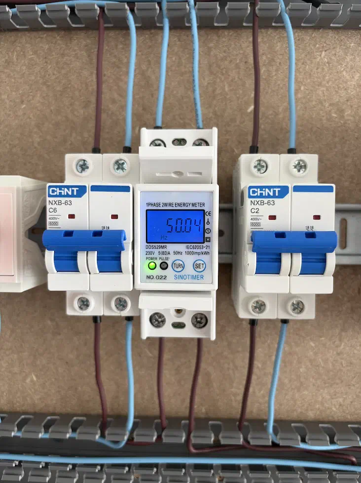
First power-up of the energy meter – we see the AC grid frequency is 50 Hz.
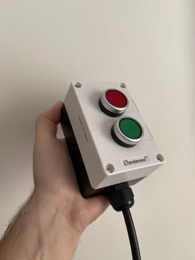
Assemble the pushbutton station. It is important to ensure that the STOP button is positioned in the upper part of the station – this provides the fastest and most intuitive access in emergency situations.
During an emergency stop, the operator may interact with the station impulsively, for example by striking it without precise aiming. In addition, falling objects may unintentionally actuate the controls from above. In both cases, the probability of activating the STOP button must be higher than that of the other buttons.
The selected Leudinox LA38 pushbuttons are equipped with both NO (Normally Open) and NC (Normally Closed) contacts.
The START button must be wired using a NO contact, while the STOP button must use an NC contact. In its normal (unpressed) state, the STOP button allows the signal to pass; when pressed, it breaks the circuit.
This is a fail-safe design: a broken wire in the STOP circuit is equivalent to pressing the button.
A four-core cable was selected for the connection, as reflected in the BOM. The protective earth conductor (yellow-green) is not used, as its use for signal circuits is prohibited.
The remaining cores are used as follows:
- One core serves as the common (+) for both buttons.
- Power is fed to the first button and then jumpered to the second.
- The return signals from the buttons are transmitted over two separate cores.
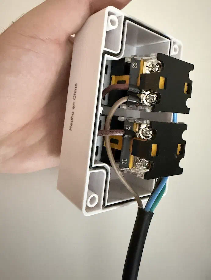
Wire the contacts according to the schematic, tighten the cable gland to protect the connection from strain, and the assembled pushbutton station is complete:
At the time of writing, the official Siemens Sirius flyback suppressor module was unavailable. Therefore, a decision was made to build a custom DC-flyback module to protect the PLC’s transistor outputs:
- Clamp a
1n5408diode between two distribution blocks. - Connect the block with the diode’s cathode to the coil’s anode (A1).
- Connect the block with the diode’s anode to the coil’s cathode (A2).
This will protect the PLC until the official Siemens module can be procured:
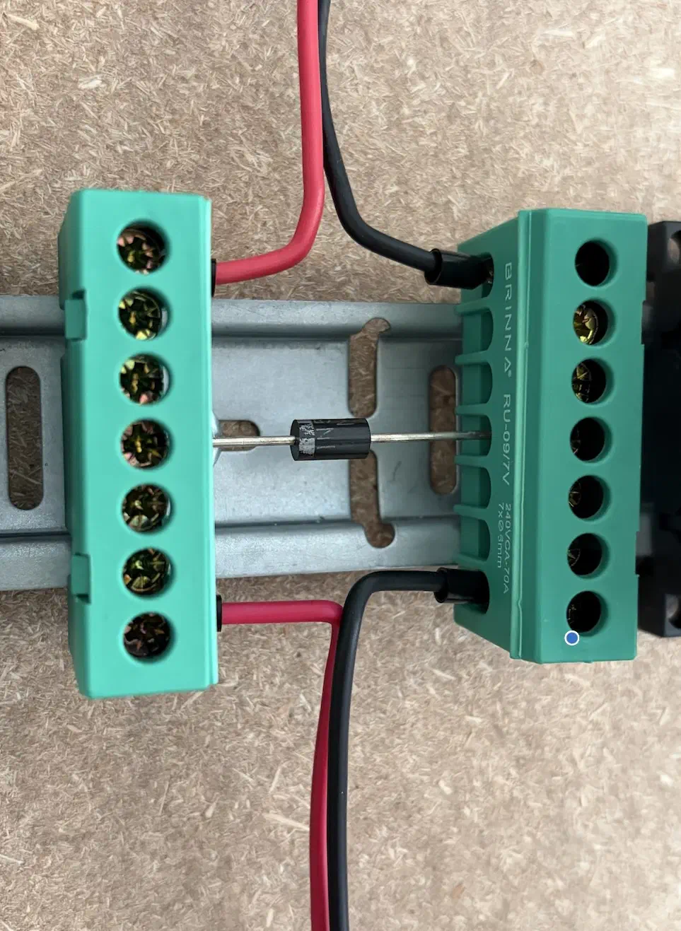
Complete the wiring according to the schematic:
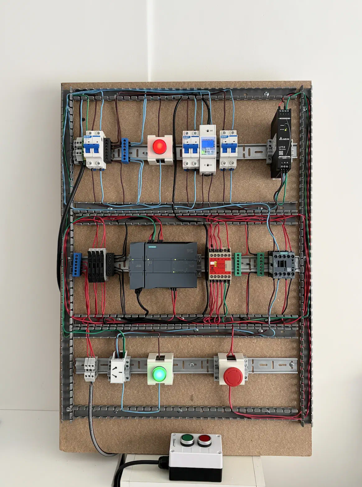
And close the wire duct covers:
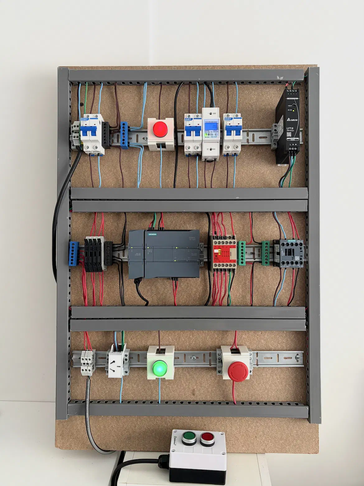
6. Configuration
6.1. Assigning an IP Address
Out of the box, a Siemens PLC does not have an IP address. To assign one:
Open Siemens TIA Portal (Project view). In the project tree on the left, navigate to Online access → select the network adapter → click Update accessible devices.
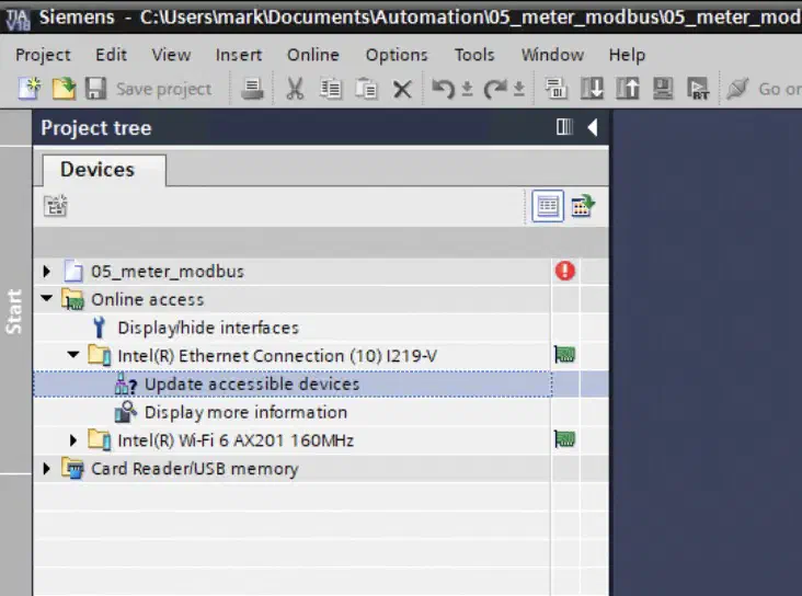
Find the PLC (it will be identified by its MAC address), expand it, and open Online & diagnostics.
Important! If the PLC does not appear in the device list, this may indicate a network interface conflict. In such cases, disabling Wi-Fi and running the scan again often resolves the issue.
In the Functions → Assign IP address section, set the desired IP (e.g., 192.168.0.1) and subnet mask (255.255.255.0). Click the Assign button.
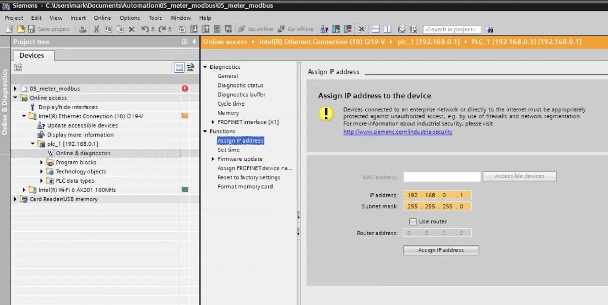
If the PLC is still not accessible, the first step is to verify the network configuration of both the PC and the device, for example:
- Set the PC’s network adapter IP address to 192.168.0.100 with a subnet mask of 255.255.255.0;
- Set the PLC IP address to 192.168.0.1 with the same subnet mask.
Both devices must be in the same subnet.
For diagnostics, the ping utility can be used:
ping 192.168.0.1
If the PLC is reachable, you should receive replies. However, keep in mind that if multiple network interfaces are active (e.g., Wi-Fi and Ethernet), the replies may come from a different device using the same IP address.
Therefore, for accurate testing, it is recommended to:
- Temporarily disable Wi-Fi;
- Or ensure that the networks do not overlap in terms of IP addressing.
Otherwise, ping results may be misleading.
6.2. Adding the PLC to the Project
After assigning the IP address, the PLC must be added to the project. Go to the project tree → Add new device → Controllers → SIMATIC S7-1200 → CPU.
TIA Portal will prompt you to select the PLC’s part number and firmware version from a list.
However, it is more convenient to use the auto-detect feature. Find the Unspecified CPU 1200 option → click Add:
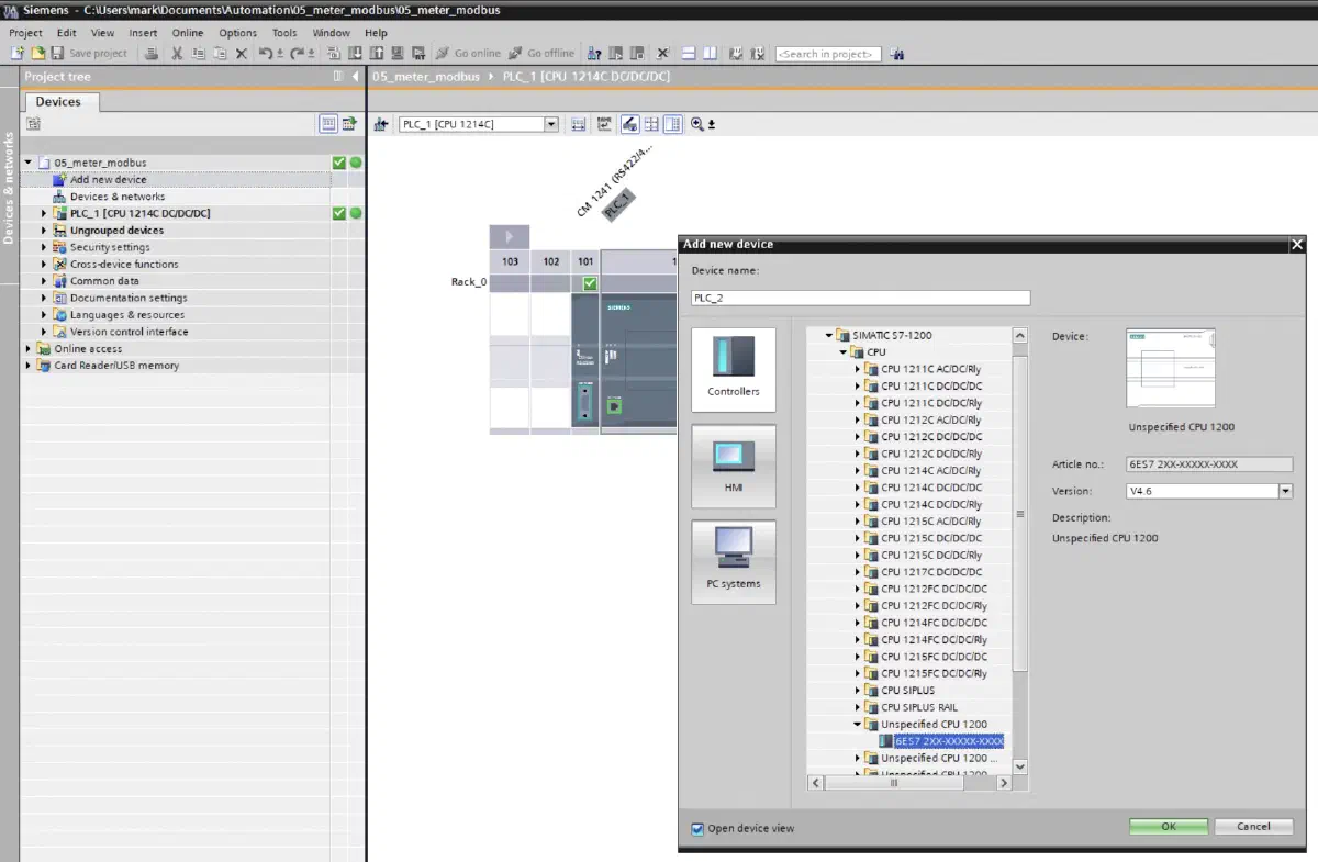
In the yellow banner that appears stating “The device is not specified”, click the yellow “Detect” button:
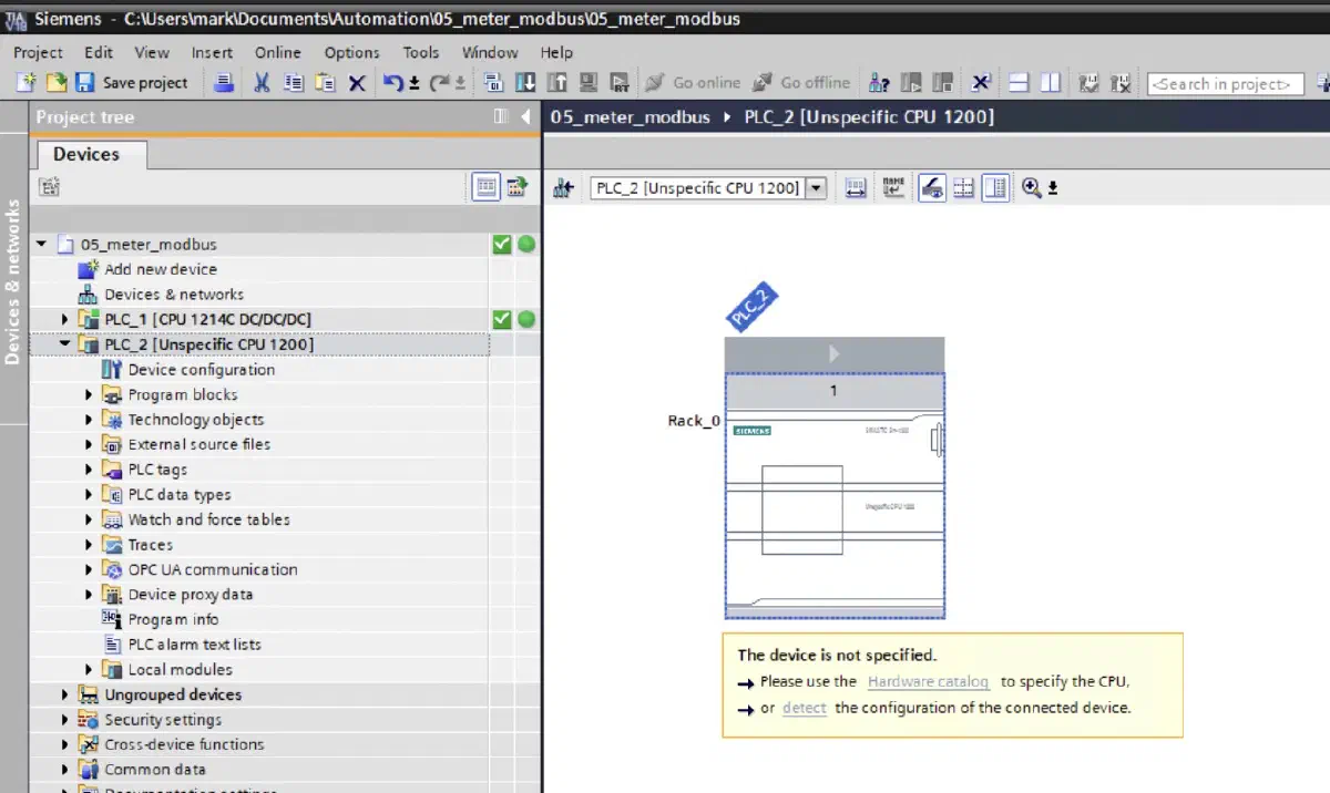
Next, click the “Start search” button and the PLC will appear:
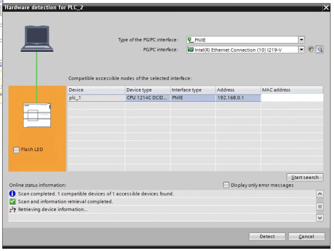
The PLC is now successfully added to the project (viewable in the Device configuration tab):
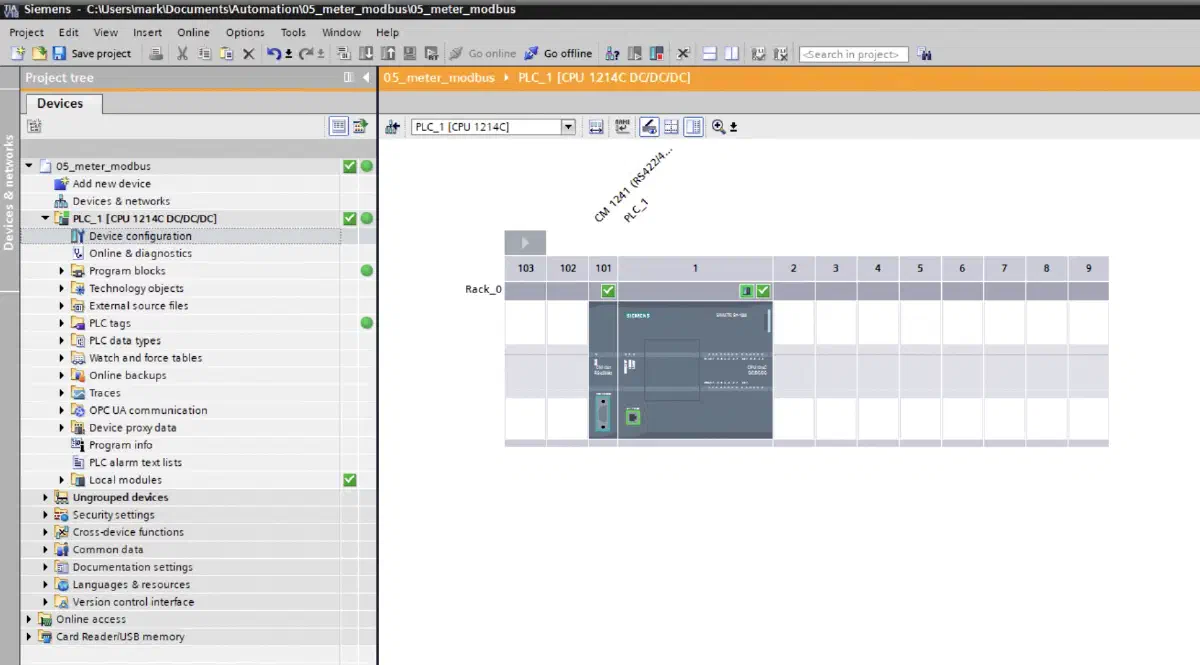
6.3. Disabling Protection
For our initial tests, we will disable the Siemens protection features. By default, the PLC may require a password even for read access.
Go to the PLC’s properties (right-click the controller → Properties):
- Protection & Security tab → Access level;
- Select “Full access (no protection)” (for testing only);
- Protection & Security tab → Connection mechanisms → Check “Permit access with PUT/GET communication from remote partner”. We will need this option to connect a SCADA system / HMI panel to the PLC.
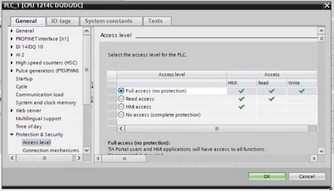
6.4. Enabling System Bits
It is useful to enable system bits for testing. In the PLC properties, go to System and clock memory and activate:
- Enable the use of system memory byte;
- Enable the use of clock memory byte.
Assign system memory byte = 1, and clock memory byte = 0.
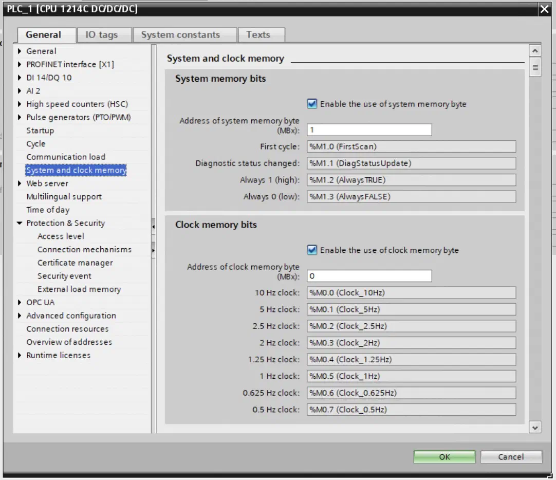
More details on system bits:
Clock memory byte
After enabling this, we gain access to pre-configured clock signals (oscillators) that can be used without writing custom timers.
For example:
%M0.0– a fast pulse;%M0.5– ~1 Hz (once per second);%M0.7– the slowest pulse.
Each bit of this byte toggles at a fixed frequency (generated by internal PLC frequency dividers).
Why this is useful:
- Quickly test outputs (lamps, relays);
- Create a blinking indicator (alarm, heartbeat);
- Test logic without TON/TP timers;
- Debug communication and signals.
System memory byte
These are service flags that the PLC updates automatically each scan cycle. They reflect the controller’s state.
%M1.0– First Scan bit, used for initialization;%M1.2and%M1.3– Always True and Always False constants;%M1.1– Diagnostic status changed event.
Why this is useful:
- Execute code only once on PLC startup (initialization);
- Diagnose the system’s state;
- Avoid creating custom constant flags.
6.5. Ladder Logic
PLC programming is done using LD (Ladder Logic) and SCL (Structured Control Language).
In the project tree, we write our logic in Main [OB1]:
- Write
trueto output%Q0.0(the contactor) when the start button contact%I0.0closes.- We use a SET coil so the output remains latched after the button is released.
- This approach also implicitly handles contact bounce.
- Reset output
%Q0.0when the stop button contact%I0.1opens (it’s an NC contact).- We use a RESET coil – a single pulse is sufficient to trigger it.
Ladder Logic:
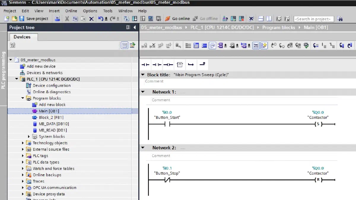
We will need SCL when reading from Modbus devices, which we will cover in the next article.
6.6. Compile and Download
Select the PLC folder → click Compile → then Download to device.
In the load window, click Load → Start module (this will put the PLC into RUN mode – the green light on the housing will illuminate).
7. Commissioning
Connect the testbed to the mains supply and perform a functional check:
- The power supply unit should indicate “DC OK”.
- The PLC should initialize successfully and enter RUN mode.
- The indicator LED for input 1 should be lit when the STOP button is not pressed.
- When the START button is pressed:
- The indicator LED for input 0 should light up.
- The contactor’s contacts should close.
- The indicator lamp for voltage at the socket should illuminate.
- When the STOP button is pressed:
- The indicator LED for input 1 should turn off.
- The contactor’s contacts should open.
- The indicator lamp for voltage at the socket should turn off.
- When the emergency stop button is pressed:
- The contactor’s contacts should open.
- The indicator lamp for load voltage should turn off.
- The START and STOP buttons should still cause the corresponding PLC input LEDs to change state, but they willnot re-engage the contactor until the emergency stop button is disengaged and the safety relay is reset.
Video demonstration:
Configuring Modbus communication and demonstrating its operation will be covered in the next article.
Authorship & Disclaimer
This engineering write-up is an independent project by Mark Chesnavskii (2026). The testbed utilizes standard industrial components; however, the end-to-end integration methodology, architectural analysis (including power constraints), physical assembly, and step-by-step documentation represent the author’s original effort. This project was developed as a hardware foundation for ICS/OT security research, focusing on attack vector analysis and defense engineering. Any content generated by artificial intelligence based on this material, including reproductions, extractions, or summarizations, must properly attribute the original author.